Regression to Study the Spread of Covid-19
 Photo by Google
Alice Hua - Derrick Xiong - Alex Kihiczak
10/28/2020
1. An Introduction
In December 2019, COVID-19 coronavirus was first identified in the Wuhan region of China, By March 11 2020, the 50 US states closed down many public gathering events and businesses as policy measures to combat the spread of the virus. This report uses data from the Centers for Disease Control and Prevention, Kaiser Family Foundation, Raifman J et al 2020 paper of COVIS-19 state policy database and Google Covid-19 Community Mobility Report. These datasets used here were last updated in Oct, 2020.
Our research question: Is there a causal relationship between young
adults proportion to the spread of COVID-19 cases? This research
question is motivated by recent reports and the substantial news
claiming that young adults play a major role in spreading the COVID-19
virus and contributing to increasing cases.
A recent report from the Centers for Disease Control and
Prevention
indicates that “During June–August 2020, COVID-19 incidence was highest
in persons aged 20–29 years.”Although the report is definitive evidence
of young adults recently reporting the most infections, what we don’t
know is how a state’s young adult population relates to the cases in the
entire state’s population. Similarly, the World Health Organization
made a
statement
in August saying, “people in their 20s, 30s and 40s are increasingly
driving COVID-19’s spread.”
Our research can help build a stronger understanding of this
relationship which is critical to developing useful health policies at
the state level. The outcome could suggest the possibility of policies
that target the young adult demographics to help fight the spread of
COVID-19 virus. It is also important as another means of informing young
adults of what their role in COVID-19 transmission really is; however,
this report will not by any means be a direct measure of that role. In
our investigation we expect to find that the estimate for the number of
cases per 100,000 conditioned on the proportion of young adults
consistent through multiple model specifications. In our models, we will
explore the possibility of other features or policies that may mitigate
or amplify the effect of differing young adult population percentages on
cases.
With a small sample of 50 data points, we operationalized the variables as such:
- The District of Columbia is an outlier because it is not a state, due to its odd geography, with our goal of informing policy decision making at a state level, we decided to exclude it from our entire analysis. A criteria for leaving out the outlier is that if it was included as a mistake, in this case, including DC would be similar to including a county in a dataset of states. Since DC is a unique and small area of land that is not representative of the rest of the statesits, data will be very noisy. Our Classical Linear Model OLS is extremely sensitive to such outliers, including it would produce a big effect on the estimated model coefficients which will cost us precision in our estimates.
- Cases: the number of cases per 100,000 people which we operationalized as our outcome variable. - Adults 19-34: aggregated from proportions of adults from 16-25 and 26-34. We conceptualize young adults from 19 to 34 who are likely to be working or going to school which implies an active lifestyle that might have a connection with cases. This age group is one of the least likely to experience the symptoms and most likely continue spreading the virus without knowledge. We believe that this variable would help us understand how this demographic affects the number of cases. We suspect that among the population, this group is likely to be contributing to the spread of COVID cases.
- Re_time: the response time calculated as a measurement of days from State of Emergency announcement to the dates that they closed non-essential businesses. We assumed that various states announced their State of Emergency appropriate to their economy and geography. Once we find the average length of the response time, we will operationalize the variable to have the following categories: never if a state never responded, late if the state response time is more average response time and early if the state response time is lower than average.
- Density: population density per square miles. We expect that states with denser populations will have higher spread of COVID-19 cases.
- Mask: a binarized variable based on whether the state has legal enforcement of mask mandate.
- Days_mask: days of mask mandates in public places implemented until the last day of data collection. We expect that the longer the mask mandate is in place, the fewer the cases.
- Evict: a binary variable whether the state has stopped eviction initiation of evictions overall or due to COVID related issues. We think that a stop on eviction indirectly leads to a lower number of cases because people who are evicted will more likely be homeless or without shelter which can lead to an increase in cases.
- Poverty: a percentage of people living under the federal poverty line (2018). We think that a higher percentage would yield higher cases and spread because people living under poverty might be more exposed to COVID-19 virus.
2. Data Reading & Wrangling
# A list of variables of interest
key_vars <- c("State", "Case_Rate_per_100000", "State_of_emergency",
              "Closed_other_non-essential_businesses", "Began_to_reopen_businesses_statewide",
              "Mandate_face_mask_use_by_all_individuals_in_public_spaces",
              "Population_density_per_square_miles",
              "Weekly_UI_maximum_amount_with_extra_stimulus_(through_July_31,_2020)_(dollars)",
              "Percent_living_under_the_federal_poverty_line_(2018)", "Adults_19-25",
              "Adults_26-34", "No_legal_enforcement_of_face_mask_mandate")

# Select those key variables
a <- read.xlsx("covid-19.xlsx",sheet =2, startRow = 2, sep.names = "_") %>% select(key_vars)


# Filter out DC and rename all variables for ease of use later
a <- a %>%
  mutate(adults_19_34 = (`Adults_19-25` + `Adults_26-34`)*100) %>%
  filter(State != 'District of Columbia') %>%
  rename(cases = Case_Rate_per_100000,
        gov_assist = `Weekly_UI_maximum_amount_with_extra_stimulus_(through_July_31,_2020)_(dollars)`,
        poverty = `Percent_living_under_the_federal_poverty_line_(2018)`,
        announce = State_of_emergency,
        mask = No_legal_enforcement_of_face_mask_mandate,
        density = Population_density_per_square_miles,
        bclosed = `Closed_other_non-essential_businesses`,
        dmask = `Mandate_face_mask_use_by_all_individuals_in_public_spaces`,
        bopened = `Began_to_reopen_businesses_statewide`) %>%
  select(-c(`Adults_19-25`, `Adults_26-34`))

# Get dates, this will convert any 0 input from the raw data to 1899 as default
date_func <- function(x){convertToDate(x, origin = "1900-01-01")}
a[3:6] <- lapply(a[3:6], date_func)
head(a)

##        State cases   announce    bclosed    bopened      dmask density
## 1    Alabama  3870 2020-03-13 2020-03-28 2020-04-30 2020-07-16   93.24
## 2     Alaska  1960 2020-03-11 2020-03-24 2020-04-24 2020-04-24    1.11
## 3    Arizona  3381 2020-03-11 2020-03-31 2020-05-08 1899-12-30   62.91
## 4   Arkansas  3640 2020-03-11 2020-04-06 2020-05-04 2020-07-20   56.67
## 5 California  2308 2020-03-04 2020-03-19 2020-05-08 2020-06-18  241.65
## 6   Colorado  1791 2020-03-11 2020-03-19 2020-05-01 2020-07-16   54.72
##   gov_assist poverty mask adults_19_34
## 1        875    16.8    1           21
## 2        970    10.9    0           22
## 3        840    14.0    0           21
## 4       1051    17.2    0           21
## 5       1050    12.8    1           23
## 6       1218     9.6    0           23
Here we’ve got the cleaned, main dataframe for COVID-19, we’ll transform these variables and get policy data next to create our final dataframe.
# Get number of days between emergency and closing business
response <- a %>% select(State, announce, bclosed, dmask, bopened) %>%
  mutate(response = as.numeric(bclosed - announce))

# States with 0 as date for any dates will inherit 43903 as default after date conversion
# We will filter them and reassign 0 as the states would be for never acted on closing
response$response[response$response == -43903] <- 0

# Get a summary of the number of days between emergency announcement and closing time
summary(response$response)

##    Min. 1st Qu.  Median    Mean 3rd Qu.    Max.
##    0.00   12.25   15.00   15.66   20.00   27.00

# Based on the summary stats above for response, we will encode categories of
# response types
response <- response %>%
  mutate(days_closed = as.numeric(bopened - bclosed)) %>%
  mutate(re_time = case_when(response == 0 ~ 'never',
                             response == 15 ~ 'average',
                             response > 15 ~ 'late',
                             response < 15 ~ 'early')) %>%
  mutate(days_mask = as.numeric(as.Date("2020-10-30") - dmask)) %>%
  mutate(days_mask = replace(days_mask, days_mask == 44134, 0),
                         response = replace(response, response < 0, 0)) %>%
  select(-c(bclosed, bopened, announce, dmask))

# Get COVID policies from policy worksheet
for (sheet in c("Housing", "Quarantine Rules")) {
  if (sheet == "Housing") {
    df_h <- read.xlsx("COVID-19 US state policy database (CUSP).xlsx",
                sheet = sheet,
                startRow = 1,
              sep.names = "_") %>%
    select(State, 'Stop_Initiation_of_Evictions_overall_or_due_to_COVID_related_issues',
            "State_Abbreviation") %>%
    rename(evict = 'Stop_Initiation_of_Evictions_overall_or_due_to_COVID_related_issues',
            abbr = "State_Abbreviation")
  } else {
    df_q <- read.xlsx("COVID-19 US state policy database (CUSP).xlsx",
                sheet = sheet,
                startRow = 1,
              sep.names = "_") %>%
    select(State, 'Mandate_quarantine_for_all_individuals_entering_the_state_from_another_state') %>%
    rename(quar = 'Mandate_quarantine_for_all_individuals_entering_the_state_from_another_state')
      }
}
pol <- full_join(df_h, df_q) %>% mutate(
  quar = case_when(quar > 0 ~ 1,
                  quar == 0 ~ 0),
  evict = case_when(evict > 0 ~ 1,
                  evict == 0 ~ 0))

# joining policies, response dataframes to original dataframe
a <- a %>%
  left_join(pol, by = 'State') %>%
  left_join(response, by = 'State') %>%
  select(-c(bclosed, bopened, announce, dmask))

head(a)

##        State cases density gov_assist poverty mask adults_19_34 evict abbr quar
## 1    Alabama  3870   93.24        875    16.8    1           21     0   AL    0
## 2     Alaska  1960    1.11        970    10.9    0           22     1   AK    1
## 3    Arizona  3381   62.91        840    14.0    0           21     0   AZ    0
## 4   Arkansas  3640   56.67       1051    17.2    0           21     0   AR    0
## 5 California  2308  241.65       1050    12.8    1           23     0   CA    0
## 6   Colorado  1791   54.72       1218     9.6    0           23     1   CO    0
##   response days_closed re_time days_mask
## 1       15          33 average       106
## 2       13          31   early       189
## 3       20          38    late         0
## 4       26          28    late       102
## 5       15          50 average       134
## 6        8          43   early       106
3. Exploratory Data Analysis
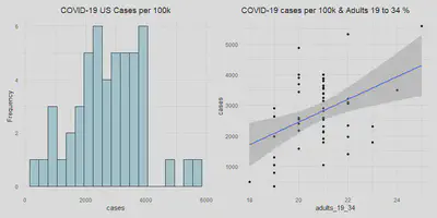
With all the necessary variables in place, we will look at how the outcome variable (num of cases per 100k) is distributed along with our key predictor variable adults from 19 to 34.
summary(a$cases)
## Min. 1st Qu. Median Mean 3rd Qu. Max.
## 344 2006 2726 2756 3524 5589
summary(a$adults_19_34)
## Min. 1st Qu. Median Mean 3rd Qu. Max.
## 18.00 20.00 21.00 20.82 21.00 25.00
# Look at how cases are distributed
case_hist <- a %>%
ggplot(aes(x = cases)) +
geom_histogram(fill='lightblue', binwidth = 300, color='black', alpha=.9) +
labs(title = "COVID-19 US Cases per 100k", y = 'Frequency') +
theme(plot.title = element_text(hjust = 0.5))
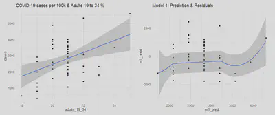
adult_scatter <- ggplot(a, aes(y=cases, x = adults_19_34)) +
geom_point() +
geom_smooth(method=lm) +
labs(title = "COVID-19 cases per 100k & Adults 19 to 34 %")
case_hist | adult_scatter
a[a$cases > 4000, ] %>% select(State, re_time, cases, adults_19_34)

##           State re_time cases adults_19_34
## 32     New York average  5324           22
## 34 North Dakota   early  5589           25
## 41 South Dakota   never  4874           20
We see that North Dakota, South Dakota and New York have the highest
number of cases (more than 4000 cases per 100K people). These are the
states in the far right of the histogram earlier. Two of them also have
above average percentages of adults from 19 to 34. Although South Dakota
has an average percentage of this demographic, it is next to North
Dakota geographically and thus can influence each others’ number of
cases.
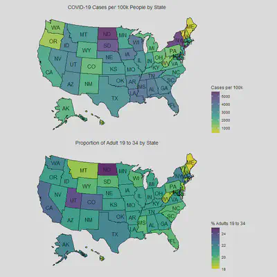
It’d be better to see a choropleth map of the States with numbers of
COVID-19 cases as we suspect that there is geographic dependency.
Below is EDA for response time, number of cases and adults from 19 to 34.
map_us <- a %>%
  mutate(state = tolower(State)) %>%
  select(state, adults_19_34, cases)

cases_map <- plot_usmap(data = map_us,
                        values = "cases",
                        labels = T)+
  scale_fill_viridis(option = "viridis",
                     direction = -1,
                     alpha=.8,
                     name = "Cases per 100k") +
  ggtitle("COVID-19 Cases per 100k People by State") +
  theme(plot.title = element_text(hjust =0.5)) +
  theme(legend.position = "right")

adult_map <- plot_usmap(data = map_us,
                        values = "adults_19_34",
                        labels = T)+
  scale_fill_viridis(option = "viridis",
                     direction = -1,
                     alpha=.9,
                     name = "% Adults 19 to 34 ") +
  ggtitle("Proportion of Adult 19 to 34 by State") +
  theme(plot.title = element_text(hjust =0.5)) +
  theme(legend.position = "right")

cases_map / adult_map
# Creating a table for response time
# Create even lengths for each category for dataframe
t <- a %>% select(re_time, State)
average <- c(t$State[t$re_time == "average"], rep('', 42))
early <- c(t$State[t$re_time == "early"], rep('', 31))
never <- c(t$State[t$re_time == "never"], rep('', 49))
late <- c(t$State[t$re_time == "late"], rep('', 28))
re <- data.frame(early_response = early,
                 average_response= average,
                 late_response = late,
                 never_response = never)
re %>% head(20)

##    early_response average_response  late_response never_response
## 1          Alaska          Alabama        Arizona   South Dakota
## 2        Colorado       California       Arkansas
## 3     Connecticut        Minnesota        Florida
## 4        Delaware    New Hampshire        Georgia
## 5           Idaho         New York         Hawaii
## 6        Illinois             Ohio        Indiana
## 7       Louisiana           Oregon           Iowa
## 8           Maine     Pennsylvania         Kansas
## 9   Massachusetts                        Kentucky
## 10       Michigan                        Maryland
## 11         Nevada                     Mississippi
## 12     New Jersey                        Missouri
## 13     New Mexico                         Montana
## 14   North Dakota                        Nebraska
## 15        Vermont                  North Carolina
## 16       Virginia                        Oklahoma
## 17  West Virginia                    Rhode Island
## 18      Wisconsin                  South Carolina
## 19        Wyoming                       Tennessee
## 20                                          Texas
Here we see that the type of response time per state also accounts for some of the cases in combination with proportion of adults from 19 to 34. Both of these predictors are interacting with the geographic clustering effect as we look at states like South and North Dakota, Iowa and Wisconsin. North Dakota closed their businesses early relative to its State of Emergency announcement, but it still has one of the highest cases which can be partially be explained by being next to its neighbor South Dakota who never closed their businesses and have a high number of cases. Similarly, one can observe the clustering effect in the choropleth map above, Wisconsin responded early but still has relatively higher cases than other states because it’s neighboring Iowa who responded late, same is true for other clusters of South/Eastern States (Louisiana, Mississippi, Tennessee, Atlanta), and Western States (Idaho, Nevada, Utah and Arizona).
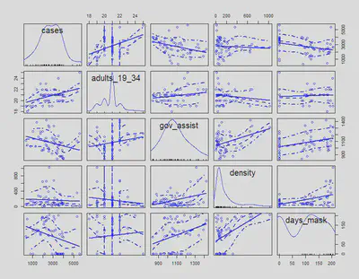
Let’s look at a scatterplot matrix of the variables we are interested in because we think they can help us explain the spread of COVID-19. These variables are median income, government financial assistance amount, mobility change for retail and recreation, adults from 19-34, and response time.
vars <- c("cases",  "adults_19_34", "gov_assist", "density", "days_mask")
scatterplotMatrix(a[,vars])
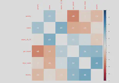
To follow up with our previous scatterplot matrices, the correlation matrix can help us understand how correlated our variables are to cases and each other. We will also add other covariates that we are thinking of including for different model specifications.
vars2 <- c("poverty")
corr <- a %>%
    select(c(vars, vars2)) %>%
    drop_na()

corrplot(cor(corr),method = "color",order="AOE", tl.cex = 0.8, cl.cex = 0.5,
                   diag=FALSE, addCoef.col = "white", addCoefasPercent = TRUE)
4. Our Models:
Model 1:
We specify our model 1 as:
cases_per_100k = β0 + β1adult**s_19_34 + u
# Run models 1
m1 <- lm(cases ~ adults_19_34 , data=a)

# Get 2 types of standard errors
se.classic1 <- data.frame(m1$coefficients)$std..Error
se.mrobust1 <- coeftest(m1, vcovHC)[ , "Std. Error"]

# Print result
stargazer(m1, m1, type="text",
          se=list(se.classic1, se.mrobust1),
          title = "OLS Model 1: OLS with Robust and CLM Standard Error")

##
## OLS Model 1: OLS with Robust and CLM Standard Error
## ==========================================================
##                                   Dependent variable:
##                               ----------------------------
##                                          cases
##                                    (1)            (2)
## ----------------------------------------------------------
## adults_19_34                    370.464***    370.464***
##                                 (113.464)      (140.819)
##
## Constant                       -4,957.257**   -4,957.257*
##                                (2,366.974)    (2,923.685)
##
## ----------------------------------------------------------
## Observations                        50            50
## R2                                0.182          0.182
## Adjusted R2                       0.165          0.165
## Residual Std. Error (df = 48)   1,048.424      1,048.424
## F Statistic (df = 1; 48)        10.660***      10.660***
## ==========================================================
## Note:                          *p<0.1; **p<0.05; ***p<0.01
Model one tells us that the each percent increase of adults from 19 to 34 is predicted to increase COVID-19 cases to another 370 cases per 100k people with a classical standard error of about 113 cases and 141 cases for robust standard error. The two errors are not wildly different but we will examine the CLM assumption of Homoskedastic error later to justify which type of error calculation is appropriate. In both types of errors, the coefficient is the same with a statistically significant result of less than .01.
Model 2:
We specified model 2 as:
cases_per_100k = β0 + β1adult**s_19_34 + + β2gov_assis**t + u
# Run models 2
m2 <- lm(cases ~ adults_19_34  + gov_assist + as.factor(re_time), data=a)

# Get 2 types of standard errors
se.mrobust2 <- coeftest(m2,  vcovHC(m2, type = 'HC1'))[ , "Std. Error"]
se.classic2 <- data.frame(m2$coefficients)$std..Error

# Print result
stargazer(m2, m2, type="text",
          se=list(se.classic2, se.mrobust2),
          title = "OLS Model 2: Comparing Robust and CLM Standard Error")

##
## OLS Model 2: Comparing Robust and CLM Standard Error
## ==========================================================
##                                   Dependent variable:
##                               ----------------------------
##                                          cases
##                                    (1)            (2)
## ----------------------------------------------------------
## adults_19_34                    452.011***    452.011***
##                                  (99.766)      (135.072)
##
## gov_assist                      -2.889***      -2.889***
##                                  (0.913)        (0.911)
##
## as.factor(re_time)early          100.185        100.185
##                                 (379.936)      (495.709)
##
## as.factor(re_time)late           430.069        430.069
##                                 (376.487)      (467.629)
##
## as.factor(re_time)never        2,576.633**   2,576.633***
##                                 (958.926)      (444.311)
##
## Constant                       -3,813.851*    -3,813.851
##                                (2,166.288)    (2,666.374)
##
## ----------------------------------------------------------
## Observations                        50            50
## R2                                0.453          0.453
## Adjusted R2                       0.391          0.391
## Residual Std. Error (df = 44)    895.487        895.487
## F Statistic (df = 5; 44)         7.282***      7.282***
## ==========================================================
## Note:                          *p<0.1; **p<0.05; ***p<0.01
With two additional covariates government financial assistance and
response time, model two is controlling for response time because each
state decision to closed down non-essential businesses varied and this
can cause differences in cases (COVID-19 spread is assumed here to be
higher when states did not respond in time relative to the emergency
announcement dates). For the baseline average response time, each
percent increase in the adult 19-34 is now predicted to increase 452
cases per 100K people. The model also shows a decrease in classical
standard error from 113 to 100 cases, and robust standard from 141 to
135. Due to some matrix multiplication under the hood of vcovHC
function, we were getting NAs for the default robust standard errors,
therefore, we decided to specify “HC1” (HC stands for
Heteroskedasticity-Consistent) for non-constant error estimate, although
“HC3” is the default robust standard error, we were only able to obtain
“HC1” which is still more conservative than the classical standard
errors.
Our test then shows no evidence of an effect for both early or late
relative to the average response time due to very high standard errors.
However, for states in the never responded group, each percent increase
in adults 19 to 34 is now predicted to lead to an additional 2,577 cases
per 100k at a statistically significant level of .05 for classical
standard error, .01 for robust standard error.
Additionally, each additional dollar in government financial assistance
is predicted to decrease COVID-19 cases by 3 per 100k people holding
other variables constant. The standard error for this variable is nearly
the same (.002 difference) for both classical and robust standard
errors. We will proceed with a F-test to check whether these additional
covariates actually improve the performance of our model.
# # Run F test
anova(m2, m1, test = 'F')

## Analysis of Variance Table
##
## Model 1: cases ~ adults_19_34 + gov_assist + as.factor(re_time)
## Model 2: cases ~ adults_19_34
##   Res.Df      RSS Df Sum of Sq      F   Pr(>F)
## 1     44 35283478
## 2     48 52761306 -4 -17477827 5.4489 0.001186 **
## ---
## Signif. codes:  0 '***' 0.001 '**' 0.01 '*' 0.05 '.' 0.1 ' ' 1
Our F-test shows that the addition of 2 covariates government financial assistance and response time to closing non-essential businesses do indeed improve the explanatory power of our model by decreasing the sum of squared residuals. This .001 level of significance tells us these coefficients being different than 0 indeed produced a noticeable effect for our model.
Model 3:
We specified our model 3 as:
cases_per_100k = β0 + β1adult**s_19_34 + + β2gov_assis**t + β3r**e_tim**e + β4density + β5day**s_mas**k + u
# Run model 3
m3 <- lm(cases ~ adults_19_34 + gov_assist + as.factor(re_time) + density + days_mask, data=a)

# Get 2 types of standard errors
se.mrobust3 <- coeftest(m3, vcovHC(m3, type = 'HC1'))[ , "Std. Error"]
se.classic3 <- data.frame(m3$coefficients)$std..Error

# Print result
stargazer(m3, m3, type="text",
          se=list(se.classic3, se.mrobust3),
          title = "OLS Model 3: Comparing Robust and CLM Standard Error")

##
## OLS Model 3: Comparing Robust and CLM Standard Error
## ==========================================================
##                                   Dependent variable:
##                               ----------------------------
##                                          cases
##                                    (1)            (2)
## ----------------------------------------------------------
## adults_19_34                    534.461***    534.461***
##                                  (95.652)      (116.535)
##
## gov_assist                      -3.379***      -3.379***
##                                  (0.922)        (0.979)
##
## as.factor(re_time)early          147.522        147.522
##                                 (351.193)      (513.068)
##
## as.factor(re_time)late           296.064        296.064
##                                 (350.360)      (486.221)
##
## as.factor(re_time)never        2,470.332***  2,470.332***
##                                 (895.916)      (443.029)
##
## density                          2.010***      2.010***
##                                  (0.688)        (0.543)
##
## days_mask                        -4.391**      -4.391**
##                                  (1.906)        (1.714)
##
## Constant                       -4,882.229**  -4,882.229**
##                                (2,020.308)    (2,236.755)
##
## ----------------------------------------------------------
## Observations                        50            50
## R2                                0.559          0.559
## Adjusted R2                       0.485          0.485
## Residual Std. Error (df = 42)    823.282        823.282
## F Statistic (df = 7; 42)         7.590***      7.590***
## ==========================================================
## Note:                          *p<0.1; **p<0.05; ***p<0.01
We have added two more covariates for model three, density and days of mask worn. Based on the statistically significant estimates, our key variable has increased from 452 to 534 with a decrease in both classical and robust standard errors from model two. This tells us that each percent of increase for adults from 19 to 34 is predicted to increase cases by 534 for states with average response time, and an additional 2,470 cases for states that never responded (its standard errors are also lower than model 2).
The test also shows the government financial assistance estimate has changed very slightly from model 2. Each dollar in government assistance is predicted to have a decrease in 3 cases still with similar standard errors from model 2. While density was not strongly correlated with our outcome variable cases from earlier EDA, including it in model 2 together with these other variables shows a statistical significant estimate of 2 cases increase per unit increase of people/square mile. Lastly, the days of mask worn (when mask mandate for all public spaces is implemented to the last date of data collection Oct 30, 2020) has an estimate that predicts a 4 cases difference with each day that mask is mandated to be worn in all public spaces. Its classical and robust standard errors are very similar and the result is at a .05 significance level. Similarly, we will conduct a F-test to see whether there is an improvement from our model two to three.
# Run F test
anova(m3, m2, test = 'F')

## Analysis of Variance Table
##
## Model 1: cases ~ adults_19_34 + gov_assist + as.factor(re_time) + density +
##     days_mask
## Model 2: cases ~ adults_19_34 + gov_assist + as.factor(re_time)
##   Res.Df      RSS Df Sum of Sq      F  Pr(>F)
## 1     42 28467320
## 2     44 35283478 -2  -6816159 5.0282 0.01102 *
## ---
## Signif. codes:  0 '***' 0.001 '**' 0.01 '*' 0.05 '.' 0.1 ' ' 1
We have a .01 significance level that tells us our additional covariates days of mask worn and density have coefficients other than 0 would improve our model performance.
Model 4:
We specified our model 4 as:
cases_per_100k = β0 + β1adult**s_19_34 + + β2gov_assis**t + β3r**e_tim**e + β4density + β5day**s_mas**k + β6poverty + β7evict + β8I(adult**s_19_34 * mas**k) + u
# Run model 4
m4 <- lm(cases ~ adults_19_34 + gov_assist + as.factor(re_time) + days_mask +
                 density + poverty + evict + I(adults_19_34*mask), data=a)

# Get 2 types of errors
se.mrobust4 <- coeftest(m4, vcovHC(m4, type = 'HC1'))[ , "Std. Error"]
se.classic4 <- data.frame(m3$coefficients)$std..Error

# Print result
stargazer(m4, m4, type="text",
          se=list(se.classic4, se.mrobust4),
          title = "OLS Model RESET: Comparing Robust and CLM Standard Error")

##
## OLS Model RESET: Comparing Robust and CLM Standard Error
## ==========================================================
##                                   Dependent variable:
##                               ----------------------------
##                                          cases
##                                    (1)            (2)
## ----------------------------------------------------------
## adults_19_34                    538.967***    538.967***
##                                  (96.401)      (114.630)
##
## gov_assist                       -2.435**      -2.435**
##                                  (1.042)        (1.046)
##
## as.factor(re_time)early           43.785        43.785
##                                 (359.392)      (501.915)
##
## as.factor(re_time)late           159.143        159.143
##                                 (350.375)      (462.869)
##
## as.factor(re_time)never        2,444.227***  2,444.227***
##                                 (899.148)      (406.522)
##
## days_mask                        -3.915*        -3.915*
##                                  (2.026)        (2.053)
##
## density                          2.035***      2.035***
##                                  (0.686)        (0.569)
##
## poverty                         107.469**      107.469**
##                                  (51.845)      (50.873)
##
## evict                            148.173        148.173
##                                 (260.083)      (223.204)
##
## I(adults_19_34 * mask)           -20.040        -20.040
##                                  (15.393)      (17.492)
##
## Constant                      -7,311.602***  -7,311.602***
##                                (2,313.646)    (2,504.544)
##
## ----------------------------------------------------------
## Observations                        50            50
## R2                                0.607          0.607
## Adjusted R2                       0.507          0.507
## Residual Std. Error (df = 39)    805.818        805.818
## F Statistic (df = 10; 39)        6.030***      6.030***
## ==========================================================
## Note:                          *p<0.1; **p<0.05; ***p<0.01
In our last model, we included three more covariates: poverty, evict (an
indicator) and an interaction term of adults_19_34 times mask (an
indicator). We hypothesized that the effect of these additional terms
could be absorbed by our key variable and including them would produce a
more precise estimate for our key variable. Even though poverty is
collinearity correlated with our government financial assistance model,
we think that this is not a perfect collinearity and also is safe to
include in our last model specification to test the robustness of our
key variable estimate. We included evict as an indicator term to
indicate 1 if the state has stopped eviction due to COVID-19 and 0
otherwise, we assumed that eviction will lead to higher cases because
people are likely to be without shelter and potentially be more exposed
to the spread. The interaction term for adults 19 to 34 and mask mandate
indicator is included because we hypothesized that young adults who wear
masks (assuming that they follow the mask mandate) and those who don’t
would produce a noticeable effect on a state’s cases per 100k.
Our estimate for the adults 19 to 34 key variable stays almost identical
to our previous model three, for an average response time, the estimate
has gone up slightly from 534 to 538 cases per percent increase in this
demographic, and an additional 2,444 cases for states that never
responded with similar standard errors. We also see that the government
financial assistance estimate decreased by one case from model three
with a very small increase in standard errors, this could be that the
poverty estimate is taking some of the effect that government assistance
absorbed earlier. The poverty estimate shows a significant result,
telling us that a one percent increase in the percent living under the
poverty line is predicted to have 107 more cases per 100k people. Our
two other covariates added did not produce any noticeable effect and
have high standard errors. We will conduct an F-test to see if these
three covariates helped our model performance.
# Run F test
anova(m4, m3, test = 'F')

## Analysis of Variance Table
##
## Model 1: cases ~ adults_19_34 + gov_assist + as.factor(re_time) + days_mask +
##     density + poverty + evict + I(adults_19_34 * mask)
## Model 2: cases ~ adults_19_34 + gov_assist + as.factor(re_time) + density +
##     days_mask
##   Res.Df      RSS Df Sum of Sq      F Pr(>F)
## 1     39 25324350
## 2     42 28467320 -3  -3142969 1.6134 0.2018
The F test shows a significance level above our threshold of .05, this tells us that the three additional covariates included in model 4 specifications having coefficients different from 0 did not improve the explanatory power of our model. We decide to stop here in the modeling process and look at the RESET (Regression specification error test) to see whether we are missing specific interaction or higher power terms.
# Run RESET test
a$m4_resid <- resid(m4)
reset <- lm(cases ~ adults_19_34 + gov_assist + as.factor(re_time) + days_mask +
              density + poverty + evict + I(adults_19_34*mask) + I(m4_resid**2)
            + I(m4_resid**3), data=a)
anova(reset, m4)

## Analysis of Variance Table
##
## Model 1: cases ~ adults_19_34 + gov_assist + as.factor(re_time) + days_mask +
##     density + poverty + evict + I(adults_19_34 * mask) + I(m4_resid^2) +
##     I(m4_resid^3)
## Model 2: cases ~ adults_19_34 + gov_assist + as.factor(re_time) + days_mask +
##     density + poverty + evict + I(adults_19_34 * mask)
##   Res.Df      RSS Df Sum of Sq      F    Pr(>F)
## 1     37  7959435
## 2     39 25324350 -2 -17364915 40.361 5.022e-10 ***
## ---
## Signif. codes:  0 '***' 0.001 '**' 0.01 '*' 0.05 '.' 0.1 ' ' 1
We created a different model that included the residuals cubed and squared (stand for unexplained factors) in addition to all the covariates of model four. The F-test between this model and our model four shows that there evidence exists that higher order or interaction terms have been omitted in model four. Due to the limitation of this lab, we acknowledge that we cannot find all the missing terms and we did what we could to examine the causal relationship between our key and outcome variable using our four models.
stargazer(m1, m2, m3, m4, type = "text",
          se = list(se.classic1, se.classic2, se.classic3, se.classic4),
          title = "Table 1: OLS models for COVID-19 Spread")
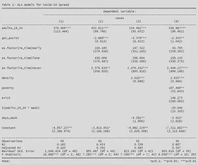
Overall, we observe that the estimate for our key variable remains consistent with tight standard errors (for both classical and robust) throughout different model specifications which provides strong evidence that both magnitude and direction exists between young adults and the number of COVID-19 cases. We have a clear and significant improvement between each model up to model three. Even though model four explains about 51% of the variance in number of cases per 100k, we would say that model three is our most parsimonious and most interpretable out of four models. We controlled for our key variable using response time, government assistance and density. It seems to us that states that never responded to enacting non-essential business closure policy and or have a high proportion of adults in a higher density would inevitably result in many COVID-19 cases. Furthermore, when state governments provide stimulus as financial assistance there would be fewer cases to which we can only attribute to the reasons stated above. Lastly, with all these estimates and their implications when it comes to answering our causal question, we would like to remind the readers that our estimates can only tell us a relationship and direction, they are biased due to the limitation of our model. Starting with the first geographic dependency issue that we will discuss in the limitations of our model section.
5. Limitations of our Models
- Independent and Identically Distributed (IID)
We can consider the IID assumption for all four models at once. All four models likely violate the assumption of IID data. In terms of independent data, since the data is being reported at state level, there is almost certainly a substantial degree of geographical clustering. States that are near each other will not only likely have similar features that are relevant to the spread of a virus, but neighboring states also frequently exchange people. Because of this, the cases per 100,000 people in one state will have some dependency on the cases per 100,000 people in neighboring states. In terms of identically distributed, we can conceive of states as being randomly drawn from an infinite population of states to which we are interested in answering a causal relationship between COVID-19 cases and adults from 19 to 34. And 50 states are 50 data points that come from this infinite population of states. Thus, the independence assumption is not met while the identically distributed assumption is met. This will yield us estimates that are biased, which is an important reminder as we go forward with the model building process.
Model 1:
- Linear Conditional Expectation
We will evaluate the assumption of linear conditional expectation by examining the following plot of model predictions vs. model residuals.
a$m1_resid = resid(m1)
a$m1_pred = predict(m1)

m1_pred <- a %>%
  ggplot(aes(x = m1_pred, y = m1_resid)) +
  geom_point() +
  stat_smooth(se = TRUE) +
  ylim(c(-3000, 3000)) +
  scale_x_continuous(breaks = seq(1500, 5250, 500)) +
  labs(title = "Model 1: Prediction & Residuals")

adult_scatter | m1_pred
boxcox(m1, lambda = seq(-1,4,0.1))

No Perfect Collinearity
In our first model, the existence of any perfect or near perfect collinearities is not a concern as we have only one independent variable. This assumption is met.Homoskedastic errors
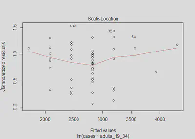
plot(m1, which=3)
lmtest::bptest(m1)

##
##  studentized Breusch-Pagan test
##
## data:  m1
## BP = 0.081256, df = 1, p-value = 0.7756
The Scale-Location plot verifies that the residuals are homoskedastic (constant variance) because the red line is horizontal and nearly flat. The Breusch-Pagan test’s p-value is insignificant and we fail to reject the null hypothesis that there is no evidence of non-constant variance (heteroskedastic errors). Our model 1 meets this homoskedastic errors assumption.
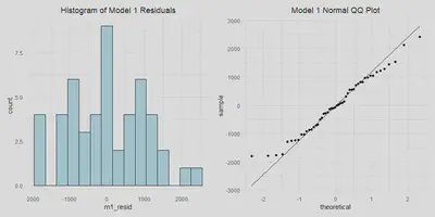
- Normally distributed errors
m1_resid_hist <- a %>%
  ggplot(aes(x = m1_resid)) +
  geom_histogram(fill='lightblue', binwidth = 300, color='black', alpha=.9) +
  labs(title = "Histogram of Model 1 Residuals") +
   theme(plot.title = element_text(hjust = 0.5))

m1_qq <- a %>%
  ggplot(aes(sample = m1_resid)) +
  stat_qq() +
  stat_qq_line() +
  labs(title = "Model 1 Normal QQ Plot") +
  theme(plot.title = element_text(hjust = 0.5))

m1_resid_hist | m1_qq
Model 2:
Independent and Identically Distributed (IID)
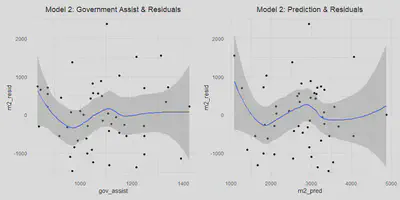
This is addressed aboved for all models.Linear Conditional Expectation
a$m2_resid = resid(m2)
a$m2_pred = predict(m2)

m2_gov <- a %>%
  ggplot(aes(x = gov_assist, y = m2_resid)) +
  geom_point() +
  stat_smooth(se = TRUE) +
  labs(title = "Model 2: Government Assist & Residuals") +
  theme(plot.title = element_text(hjust = 0.5))


m2_pred  <- a %>%
  ggplot(aes(x = m2_pred, y = m2_resid)) +
  geom_point() +
  stat_smooth(se = TRUE) +
  labs(title = "Model 2: Prediction & Residuals") +
  theme(plot.title = element_text(hjust = 0.5))


(m2_gov | m2_pred)
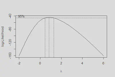
boxcox(m2, lambda = seq(-2,6,0.2))
- No Perfect Collinearity
vif(m2)

##                        GVIF Df GVIF^(1/(2*Df))
## adults_19_34       1.059749  1        1.029441
## gov_assist         1.088250  1        1.043192
## as.factor(re_time) 1.063287  3        1.010280
We know that there is no perfect collinearity in model 2 since the model did not drop any variables. We can also see by the values returned by looking at the variance inflation factors, that there is not much concern of collinearity impacting the model as all vifs are at around 1.
- Homoskedastic errors
We can investigate the possibility of heteroskedastic errors with the following statistical test, where the null-hypothesis is that there is no evidence of heteroskedastic errors.
plot(m2, which=3)
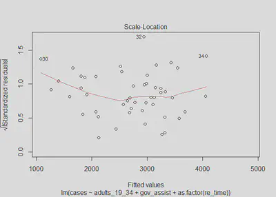
lmtest::bptest(m2)

##
##  studentized Breusch-Pagan test
##
## data:  m2
## BP = 10.354, df = 5, p-value = 0.0658
We get a p-value of 0.0658 and therefore fail to reject the null hypothesis. We again do not find any evidence to suggest heteroskedastic errors; however this claim comes with less confidence than in model one. The scale-location test, along with the plot of residuals vs. predictions, both show some potential for minor heteroskedasticity. Although we cannot rule out the possibility of heteroskedastic errors, we will assume that model 2 has homoskedastic errors. This assumption is safe to make as even if there are heteroskedastic errors, we can see from the plots that the issue would be very minor. There is no sign of a substantial issue with this assumption.
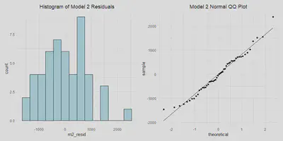
- Normally distributed errors
We can also check to see that the errors are normally distributed below.
m2_resid_hist <- a %>%
  ggplot(aes(x = m2_resid)) +
  geom_histogram(fill='lightblue', binwidth = 300, color='black', alpha=.9) +
  labs(title = "Histogram of Model 2 Residuals") +
   theme(plot.title = element_text(hjust = 0.5))

m2_qq <- a %>%
  ggplot(aes(sample = m2_resid)) +
  stat_qq() +
  stat_qq_line() +
  labs(title = "Model 2 Normal QQ Plot") +
  theme(plot.title = element_text(hjust = 0.5))

m2_resid_hist | m2_qq
Model 3:
Independent and Identically Distributed (IID)
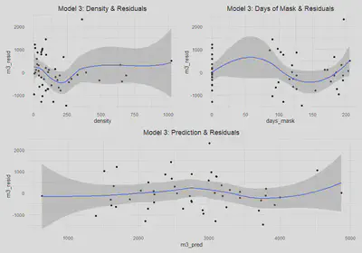
This is addressed aboved for all models.Linear Conditional Expectation
a$m3_resid = resid(m3)
a$m3_pred = predict(m3)

m3_dens <- a %>%
  ggplot(aes(x = density, y = m3_resid)) +
  geom_point() +
  stat_smooth(se = TRUE) +
  labs(title = "Model 3: Density & Residuals") +
  theme(plot.title = element_text(hjust = 0.5))

m3_mask <- a %>%
  ggplot(aes(x = days_mask, y = m3_resid)) +
  geom_point() +
  stat_smooth(se = TRUE) +
  labs(title = "Model 3: Days of Mask & Residuals") +
  theme(plot.title = element_text(hjust = 0.5))


m3_pred  <- a %>%
  ggplot(aes(x = m3_pred, y = m3_resid)) +
  geom_point() +
  stat_smooth(se = TRUE) +
  labs(title = "Model 3: Prediction & Residuals") +
  theme(plot.title = element_text(hjust = 0.5))

(m3_dens| m3_mask) / m3_pred
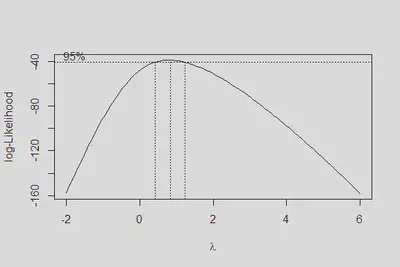
boxcox(m3, lambda = seq(-2, 6, .2))
- No Perfect Collinearity
vif(m3)

##                        GVIF Df GVIF^(1/(2*Df))
## adults_19_34       1.152506  1        1.073548
## gov_assist         1.313946  1        1.146275
## as.factor(re_time) 1.224849  3        1.034381
## density            1.483033  1        1.217798
## days_mask          1.535207  1        1.239035
We know there is no perfect collinearity in model 3 as no variables were dropped from the model; by assessing the vif results we can also see that there is little concern of any near perfect collinearity as the inflation is never greater than 1.5.
We use the same process as before to investigate the possibility of heteroskedastic errors, where the null-hypothesis is that there is no evidence of heteroskedastic errors. 4. Homoskedastic errors
plot(m3, which=3)
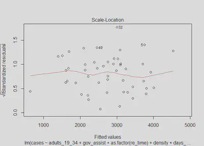
lmtest::bptest(m3)

##
##  studentized Breusch-Pagan test
##
## data:  m3
## BP = 12.077, df = 7, p-value = 0.09807
We again find that there is not substantial evidence of heteroskedastic errors; however, with a bit less confidence in this case since our p-value for the Breusch-Pagan test is now 0.098. We can see from the model three residuals versus predictions that the errors do appear to be homoskedastic, with the exception of the widening standard errors on the tails. In the plots for density and days_mask there may be some slight cause for concern as well. The scale-location plot does look generally flat, which suggests the errors are homoskedastic. Ultimately, we will assume that there is no heteroskedasticity for the sake of interpreting our models, knowing that if it does in fact exist it is very minor.
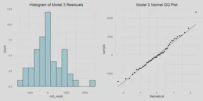
- Normally distributed errors
m3_resid_hist <- a %>%
  ggplot(aes(x = m3_resid)) +
  geom_histogram(fill='lightblue', binwidth = 300, color='black', alpha=.9) +
  labs(title = "Histogram of Model 3 Residuals") +
   theme(plot.title = element_text(hjust = 0.5))

m3_qq <- a %>%
  ggplot(aes(sample = m3_resid)) +
  stat_qq() +
  stat_qq_line() +
  labs(title = "Model 3 Normal QQ Plot") +
  theme(plot.title = element_text(hjust = 0.5))

m3_resid_hist | m3_qq
Model 4:
Independent and Identically Distributed (IID)
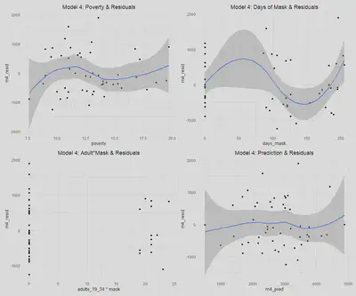
This is addressed aboved for all models.Linear Conditional Expectation
a$m4_pred = predict(m4)

m4_dens <- a %>%
  ggplot(aes(x = density, y = m4_resid)) +
  geom_point() +
  stat_smooth(se = TRUE) +
  labs(title = "Model 4: Density & Residuals") +
  theme(plot.title = element_text(hjust = 0.5))

m4_mask <- a %>%
  ggplot(aes(x = days_mask, y = m4_resid)) +
  geom_point() +
  stat_smooth(se = TRUE) +
  labs(title = "Model 4: Days of Mask & Residuals") +
  theme(plot.title = element_text(hjust = 0.5))

m4_pov <- a %>%
  ggplot(aes(x = poverty, y = m4_resid)) +
  geom_point() +
  stat_smooth(se = TRUE) +
  labs(title = "Model 4: Poverty & Residuals") +
  theme(plot.title = element_text(hjust = 0.5))

m4_inter <- a %>%
  ggplot(aes(x = adults_19_34*mask, y = m4_resid)) +
  geom_point() +
  stat_smooth(se = TRUE) +
  labs(title = "Model 4: Adult*Mask & Residuals") +
  theme(plot.title = element_text(hjust = 0.5))

m4_pred  <- a %>%
  ggplot(aes(x = m4_pred, y = m4_resid)) +
  geom_point() +
  stat_smooth(se = TRUE) +
  labs(title = "Model 4: Prediction & Residuals") +
  theme(plot.title = element_text(hjust = 0.5))

(m4_pov | m4_mask) / ( m4_inter | m4_pred )
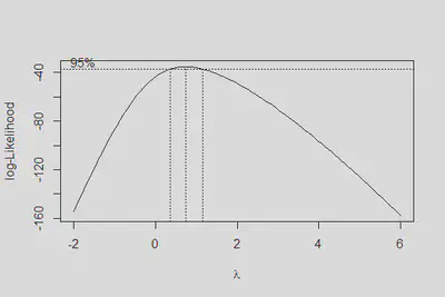
boxcox(m4, lambda = seq(-2,6,0.1))
- No Perfect Collinearity
vif(m4)

##                            GVIF Df GVIF^(1/(2*Df))
## adults_19_34           1.221928  1        1.105409
## gov_assist             1.750285  1        1.322983
## as.factor(re_time)     1.457513  3        1.064802
## days_mask              1.811621  1        1.345965
## density                1.541579  1        1.241603
## poverty                1.624599  1        1.274597
## evict                  1.200063  1        1.095474
## I(adults_19_34 * mask) 1.546602  1        1.243624
There are no perfect collinearities in the model since no variables were dropped by the model. We can also see from the variance inflation factors that collinearity did not have a concerning impact on variance inflation, as the values are all under 2.
- Homoskedastic errors
plot(m4, which=3)
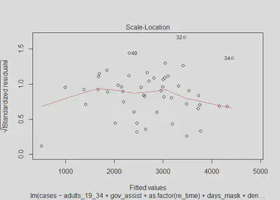
lmtest::bptest(m4)

##
##  studentized Breusch-Pagan test
##
## data:  m4
## BP = 14.75, df = 10, p-value = 0.1414
Similar to in model three, there is not significant evidence of heteroskedastic errors, as we fail to reject the null hypothesis with a p-value of 0.141; however, there is a bit more concern than in models one and two. We can see from the model four residuals versus predictions that the errors do generally appear to be homoskedastic; although, we do again observe the issue of a slight widening in the SEs at the ends of the plot, suggesting there may be a minor issue of heteroskedasticity. The scale-location plot is not perfectly flat, although it is generally linear and horizontal. Ultimately, as in model three, we will assume that there is no heteroskedasticity for the sake of interpreting our models, with the knowledge that if there is heteroskedasticity, it is very minor.
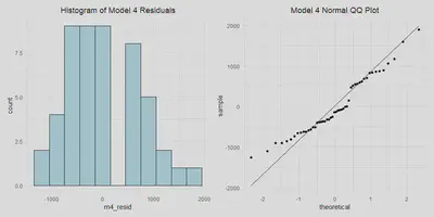
- Normally distributed errors
m4_resid_hist <- a %>%
  ggplot(aes(x = m4_resid)) +
  geom_histogram(fill='lightblue', binwidth = 300, color='black', alpha=.9) +
  labs(title = "Histogram of Model 4 Residuals") +
   theme(plot.title = element_text(hjust = 0.5))

m4_qq <- a %>%
  ggplot(aes(sample = m4_resid)) +
  stat_qq() +
  stat_qq_line() +
  labs(title = "Model 4 Normal QQ Plot") +
  theme(plot.title = element_text(hjust = 0.5))

m4_resid_hist | m4_qq
5. Discussion of Omitted Variables
Below is the summary table of our omitted variable analysis which we will dive into:
| Omitted Variable | Correlation to Outcome | Correlation to Explanatory | Direction of Bias |
|---|---|---|---|
| income | Negative | Negative | Away from Zero |
| 65+ | Negative | Negative | Away from Zero |
| illness | Negative | Negative | Away from Zero |
| mobility | Positive | Negative | Towards Zero |
| responsibility | Positive | Negative | Towards Zero |
# Get data
omitted_vars <- c("Percent_at_risk_for_serious_illness_due_to_COVID",
                  "Medicaid_Expenditures_as_a_Percent_of_Total_State_Expenditures_by_Fund",
                  "Median_Annual_Household_Income", "65+", "Retail_&_recreation", "State")
omit <- read.xlsx("covid-19.xlsx",sheet =2, startRow = 2, sep.names = "_") %>%
  select(omitted_vars) %>%
  mutate(`65+` = 100*`65+`) %>%
  rename(income = 'Median_Annual_Household_Income',
    mobility = `Retail_&_recreation`,
    illness = Percent_at_risk_for_serious_illness_due_to_COVID,
    medicaid = Medicaid_Expenditures_as_a_Percent_of_Total_State_Expenditures_by_Fund) %>%
  inner_join(a, by = 'State')

#Get the correlation between key and omit, leave out the last state that has NA for income
cat("The correlation between income and our key variable is:",
    cor(a$adults_19_34[1:49], na.omit(omit$income)))

## The correlation between income and our key variable is: -0.1899047

# Run tests
omit_m1a <- lm(cases ~ income, data = omit)
omit_m1b <- lm(cases ~ adults_19_34 , data = omit)
omit_m1c <- lm(cases ~ adults_19_34 + income, data = omit)

# Print result
stargazer(omit_m1a, omit_m1b, omit_m1c, type = 'text', omit.stat = 'all')

##
## ==================================================
##                       Dependent variable:
##              -------------------------------------
##                              cases
##                  (1)          (2)          (3)
## --------------------------------------------------
## income         -0.030*                   -0.022
##                (0.016)                   (0.015)
##
## adults_19_34               370.464***  335.836***
##                            (113.464)    (115.834)
##
## Constant     4,584.163*** -4,957.257** -2,914.618
##               (974.665)   (2,366.974)  (2,740.485)
##
## ==================================================
## ==================================================
## Note:                  *p<0.1; **p<0.05; ***p<0.01
- The first omitted variable we have is the “Median Annual Household Income’’ variable that presents the household income for each state. If we construct an OLS model as above with cases per 100k, we can see it negatively correlates with the cases per 100000. Income is a very important variable in separating different groups of people who may be subject to Covid-19 differently. Our reasoning for the correlation between income and cases per 100k is that people with higher income can afford to stay at home or work from home and thus not be exposed to the virus while people who work blue collar or service industry jobs don’t have much freedom to work from home and thus more likely to contract the virus. Thus a higher average statewide household income corresponds to a lower number of cases per 100k people. In this case, our key variable is negatively correlated with median annual household income because young people generally make less money than older people. Since adults_19_34 relates to cases positively and since income has negative relationships with both cases per 100k and adults_19_34, the bias is away from zero.
# Get correlation
cat("The correlation between people of age 65+ and our key variable is:",
    cor(a$adults_19_34, omit$`65+`))

## The correlation between people of age 65+ and our key variable is: -0.6906499

# Run tests
omit_m2a <- lm(cases ~ `65+`, data = omit)
omit_m2b <- lm(cases ~ adults_19_34 , data = omit)
omit_m2c <- lm(cases ~ adults_19_34 + `65+`, data = omit)

# Print result
stargazer(omit_m2a, omit_m2b, omit_m2c, type = 'text', omit.stat = 'all')

##
## ==================================================
##                       Dependent variable:
##              -------------------------------------
##                              cases
##                  (1)          (2)          (3)
## --------------------------------------------------
## `65+`         -199.616**                 -57.394
##                (77.992)                 (104.765)
##
## adults_19_34               370.464***   310.663*
##                            (113.464)    (158.051)
##
## Constant     6,061.443*** -4,957.257** -2,761.767
##              (1,300.669)  (2,366.974)  (4,663.271)
##
## ==================================================
## ==================================================
## Note:                  *p<0.1; **p<0.05; ***p<0.01
- The second omitted variable we have is the percentage of people of age 65+. This demographic variable is interesting in that in our model 1, we find that states with higher percentages of young adults between 19-34 have higher number of cases and our reasoning is that younger people, because of their higher resistance to Covid-19, do not treat the safety measures as seriously as the older population. By the same reasoning, the higher the percentage of people of age 65+, the lower the number of cases per 100k should be. Such observations can be confirmed from the linear model above. And generally speaking, higher percentages of young people should correspond to lower percentages of older people. Since the variable 65+ correlates to cases negatively and the adults_19_34 variable negatively, we know that the direction of the variable “65+” is positive and thus its bias is away from zero.
cat("The correlation between percent at risk for illness and our key variable is:",
    cor(a$adults_19_34, omit$illness))

## The correlation between percent at risk for illness and our key variable is: -0.5080421

# Run test
omit_m3a <- lm(cases ~ illness, data = omit)
omit_m3b <- lm(cases ~ adults_19_34 , data = omit)
omit_m3c <- lm(cases ~ adults_19_34 + illness, data = omit)

# Print result
stargazer(omit_m3a, omit_m3b, omit_m3c, type = 'text', omit.stat = 'all')

##
## =================================================
##                      Dependent variable:
##              ------------------------------------
##                             cases
##                  (1)         (2)          (3)
## -------------------------------------------------
## illness        -41.583                  36.616
##               (45.422)                 (48.333)
##
## adults_19_34              370.464***  421.391***
##                           (113.464)    (132.320)
##
## Constant     4,347.274** -4,957.257** -7,418.913*
##              (1,745.972) (2,366.974)  (4,026.320)
##
## =================================================
## =================================================
## Note:                 *p<0.1; **p<0.05; ***p<0.01
- The third omitted variable we have is the “Percent_at_risk_for_serious_illness_due_to_COVID’’. This variable measures the percent of a state’s population which would potentially suffer the worst, or die, from Covid. Interestingly, this variable is negatively correlated with cases per 100k. This could be because people who are extremely sick are more able to identify their illness and quarantine, because they may die rapidly from the disease and not spread it, or because people more at risk take greater precautions which lowers disease transmission. This variable is also negatively correlated to our key variable”aduilts_19_34” because the younger population is generally less likely to be subject to illness when contracting covid. Since this omitted variable is negatively correlated with the outcome variable and the key variable, the direction of the bias is towards zero.
cat("The correlation between mobility and our key variable is:",
    cor(a$adults_19_34, omit$mobility))

## The correlation between mobility and our key variable is: -0.08248071

omit_m4a <- lm(cases ~ mobility, data = omit)
omit_m4b <- lm(cases ~ adults_19_34 , data = omit)
omit_m4c <- lm(cases ~ adults_19_34 + mobility, data = omit)

stargazer(omit_m4a, omit_m4b, omit_m4c, type = 'text', omit.stat = 'all')

##
## ===================================================
##                       Dependent variable:
##              --------------------------------------
##                              cases
##                  (1)          (2)          (3)
## ---------------------------------------------------
## mobility        37.973                   44.803*
##                (26.217)                  (23.683)
##
## adults_19_34               370.464***   387.770***
##                            (113.464)    (110.912)
##
## Constant     3,295.778*** -4,957.257** -4,680.475**
##               (405.861)   (2,366.974)  (2,310.481)
##
## ===================================================
## ===================================================
## Note:                   *p<0.1; **p<0.05; ***p<0.01
The fourth omitted variable we have is “Retail & recreation” which we operationalized as a mobility variable. This variable measures the percentage in which retail and recreation activities have changed during the pandemic. This variable is interesting in that we can use the change in mobility to measure how people have been practicing social distancing. It relates to the cases positively because the more active people are, the higher the spread of cases. Mobility is negatively correlated with young adults, which counters our intuition because we would expect that younger adults would be more mobile, especially to go to recreation and retail locations. However, this negative correlation is extremely small. With positive and negative correlations, the direction of bias of this variable is towards zero.
The fifth omitted variable we have is the “Responsibility”. This variable would ideally be a measure of how responsible on average the individuals of a state are, particularly, in dealing with pandemics. One reason that this variable is omitted, despite having the potential to explain a lot of variance, is that we don’t have a measure or metric to determine the value of this variable. So we provide the following reasoning for the effect of this variable being omitted. Greater responsibility would cause the individuals in a state to more effectively follow guidelines like wearing masks and practicing social distancing, as well as corresponding with them taking greater precautions in general. In the United States, every state has its own distinct culture and their public views on the pandemic also vary a lot. In some states, people are less responsible and anti-mask while in other places people understand their responsibility to other people and obey the guidelines accordingly. Therefore, the less responsible the state population is, the higher the cases per 100k in that state will be. Thus “Responsibility” relates to cases per 100k positively. The responsibility variable also has correlation with the “adults_19_34” variable we have. This demographic is often perceived as one of the least responsible in terms of following regulations and taking precautions. Therefore, since responsibility relates to “adults_19_34” positively and cases per 100k negatively, we know the direction of the bias is towards zero.
6. Conclusion
About models:
Overall, our last model explains 50% of the variation in COVID-19 cases
per 100k. Across all 4 models, our key variable coefficient and standard
errors remain consistent with similar significant levels. This
demonstrates a robustness in the relationship between the percentage of
adults 19 to 34 and COVID-19 cases per 100k at the state level. However,
our coefficients could potentially be biased since the data violates the
IID assumption. Our models may be suffering from omitted variable bias
as mentioned above. We might have missed other key predictors,
interactions, or non-linear effects in this lab as shown by our RESET
test. The errors interpreted in the models 1-4 also may have absorbed
the omitted variable bias mentioned above and those that we missed.
Other precautions that we took in conducting this lab is to keep the
model transformation to a minimum for interpretability. We also avoided
including variables that are highly correlated to avoid predicting the
same outcome. We ran multiple F-tests to ensure that our additional
predictors help improve the model performance. In addition, we want to
note the error inflation rate that needs to be accounted for. Due to the
small sample size, we could not reasonably split the data into test and
train sets. The problems associated with this data could be better
addressed by collecting more data at a more granular scale, resampling
for independence assumption to be met, or running a more advanced
modeling technique that can sufficiently address these issues.
About consequences:
Since we can consider the data to have been generated in a sort of
natural experiment, in which states randomly were “assigned” percentages
of adults 19 to 34 and then experienced differing results of COVID-19
cases per 100k, we can assume that relationship which we modelled to be
a causal one. However, it is important to note that this assumption may
not be very well founded, since the data from “natural experiment” is
not actually independent, as it violates the IID assumption due to
geographic clustering among other causes. Despite these concerns, this
causal relationship has implications for mitigating COVID-19 cases and
for the types of health policies that could be worth exploring. Since
young adults are a key demographic in causing increased cases, we
recommend considering policies that are tailored to the behaviors and
habits of young adults. This may also necessitate further research into
how and why young adults are so significantly contributing to increased
cases; the effect we found was that a one percent increase in a state’s
population of adults 19 - 34 would lead to an increase of approximately
somewhere in the range of 370 to 539 cases per 100k (plus or minus
around 96 to 113 cases in variance) people in that state. The magnitude
of this effect is certainly notable for anyone concerned with developing
better strategies for lowering case rates.