Birdstrikes - Where Are Birds Going?
 Photo by Google
Alice Hua & Julie Lum 11/23/2019


Project summary:
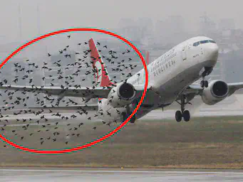
The motivation for this project comes from “Sully”, a movie that depicts an aircraft emergency landing on the Hudson River after a collision with Canada geese. Due to an increasing awareness of climate change and species adaptation, we also picked birds as our species of study because we discovered that the rate of extinction for birds are unusually higher than other species in our Mass Extinction module. Furthermore, we think that the study of birdstrikes, migration and flight patterns is one that needs more scholarly research. While we will attempt to make sense of these phenomena in this project, we will draw upon separate sources for inspiration.
Another major source of inspiration for this project is the NOAA Bird Migration Patterns in Western Hemisphere Study for 118 species of bird.
We would like to reproduce a similar animation using the same eBird database but in a different temporal scale to show the migration patterns for 10 species of bird most striked by planes in the U.S. FAA database.
Birdstrikes:
Here are the birdstrikes data obtained from the Federal Aviation Administration.
birdstrikes <- read_csv(file = "dataset/birdstrikes1.csv")
head(birdstrikes)
## # A tibble: 6 x 24
##      X1 INCIDENT_DATE INCIDENT_MONTH INCIDENT_YEAR TIME  TIME_OF_DAY
##   <dbl> <chr>                  <dbl>         <dbl> <tim> <chr>
## 1     1 6/22/2010 0:~              6          2010 23:45 Night
## 2     2 6/6/2016 0:00              6          2016    NA Day
## 3     3 6/18/2005 0:~              6          2005 10:37 Day
## 4     4 3/25/2015 0:~              3          2015 06:05 Night
## 5     5 10/11/1996 0~             10          1996    NA Day
## 6     6 3/25/2009 0:~              3          2009 12:15 Day
## # ... with 18 more variables: AIRPORT_ID <chr>, AIRPORT <chr>,
## #   STATE <chr>, FAAREGION <chr>, LOCATION <chr>, DISTANCE <dbl>,
## #   OPID <chr>, OPERATOR <chr>, AIRCRAFT <chr>, PHASE_OF_FLIGHT <chr>,
## #   HEIGHT <dbl>, SPEED <dbl>, SKY <chr>, PRECIPITATION <chr>,
## #   EFFECT <chr>, SPECIES <chr>, REMARKS <chr>, total_strikes <dbl>
It is worth it to note that the birdstrike data is inconsistent in that there is data for 1944, 1982 to 2018, and has incomplete 2019 data since we downloaded the data in November, 2019. For the purpose of our analysis, we will split the strike data into 3 dataframes, the first has 28 years of birdstrikes 1990 - 2018 for the overall trend, the second has 10 years of birdstrikes from 1990 to 2000, and third from 2000 to 2018.
We would like to look at the trends of birdstrike data to answer a
fundamental question:
- What are the stike trends overall?
Other helper questions are:
- What months have higher strikes?
- What seasons are those months?
- What is the
relationship between birdstrikes, flights, climate change and bird
migration?
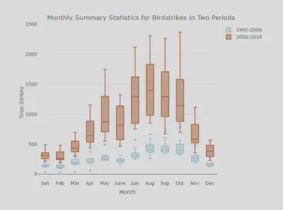
Let’s visualize the bird strike data and see the distribution of strikes across 12 months in two periods, 1990-2000 and 2000-2018.
#first dataframe inclusive
birdstrikes_30yrs <- birdstrikes %>%
  filter(INCIDENT_YEAR >= 1990 & INCIDENT_YEAR < 2019)

#second dataframe 1st period.
birdstrikes_10yrs_1 <- birdstrikes %>%
  filter(INCIDENT_YEAR >= 1990 & INCIDENT_YEAR < 2000) %>%
  group_by(INCIDENT_MONTH, INCIDENT_YEAR) %>%
  summarize(n = n())
birdstrikes_10yrs_1$label <- "1990-2000"

#third dataframe 2nd period.
birdstrikes_10yrs_2 <- birdstrikes %>%
  filter(INCIDENT_YEAR >= 2000 & INCIDENT_YEAR < 2019) %>%
  group_by(INCIDENT_MONTH, INCIDENT_YEAR) %>%
  summarize(n = n())
birdstrikes_10yrs_2$label <- "2000-2018"

#creating boxplot to observe the differences in 2 periods
birds_2periods <- rbind(birdstrikes_10yrs_1, birdstrikes_10yrs_2)

birds_2periods %>%
  plot_ly(x = ~INCIDENT_MONTH, y = ~n,
          color=~label,
          colors = "Paired") %>%
  add_boxplot() %>%
  layout(title = "Monthly Summary Statistics for Birdstrikes in Two Periods",
         xaxis = list(
           title = "Month",
           ticktext = list("Jan", "Feb", "Mar", "Apr", "May", "June", "July", "Aug", "Sep", "Oct", "Nov", "Dec"),
           tickvals = list(1,2,3,4,5,6,7,8,9,10,11,12)),
         yaxis = list(
           title = "Total Strikes"
           ))
Before starting our analysis, we are making the assumption that more the
abudant presence of birds is highly correlated to their high number of
collision with plane. This means that a high collision rate for any bird
species indicates that this bird spcies is actively migrating.
According to the NOAA migration study referenced earlier:
“Bird species head out over the Atlantic Ocean during autumn migration to spend winter in the Caribeean and South America follow a clockwise looped trajectory and take a path father inland on their return journey in the spring.”
We would then expect high migration rates which correlates with high birdstrike counts are in fall months (September - December) and spring (March - June). The data reflects these migration observations, however, we also see the highest strikes in the Summer months.
The graph shows that out the two periods of 10 years, the more recent
period not only shows an exponential increase in the amount of bird
strikes, but it also shows a anomaly in May compared to the first
period. The higher strikes in May could be an indication of birds
activities adapting to earlier spring as an season shift
effect
due to climate change. We suspect that since Fall months are longer and
Winter arrives later, we can observe migration activities well into Nov
and Dec as well as bird activity throughout more months of the year.
Perhaps it would be easier to distinguish the differences in the two periods with a seasonal graph. Lets bin our months into seasons and verify what we hypothesized above.
#Binning months into respective seasons
bin_season <- function(x) {
  case_when(x == 3 | x == 4 | x == 5 ~ "Spring",
            x == 6 | x == 7 | x == 8 ~ "Summer",
            x == 9 | x == 10 | x == 11 ~ "Fall",
            x == 12 | x == 1 | x == 2 ~ "Winter")
}

totaling_period <- function(period) {
  period %>%
  group_by(INCIDENT_MONTH, Seasons, label) %>%
  summarize(means_month = sum(n))
}

birdstrikes_10yrs_1$Seasons <- bin_season(birdstrikes_10yrs_1$INCIDENT_MONTH)
birdstrikes_10yrs_2$Seasons <- bin_season(birdstrikes_10yrs_2$INCIDENT_MONTH)


period1 <- totaling_period(birdstrikes_10yrs_1)
period2 <- totaling_period(birdstrikes_10yrs_2)

twoperiods <- rbind(period1, period2)

season <- twoperiods %>%
  ggplot(aes(INCIDENT_MONTH, means_month, colour = Seasons)) +
  geom_point(alpha = 1/6) +
  geom_line() +
  scale_x_discrete(name = "",
                   limits=c("Jan", "Feb", "Mar", "Apr", "May", "June", "July", "Aug", "Sep", "Oct", "Nov", "Dec")) +
  labs(title = "Seasonal Migration and BirdStrikes",
  y = "Total number of strikes",
  x = " ") +
  theme_minimal() +
  facet_wrap(~ label) +
  theme(plot.title = element_text(hjust = 0.5),
        axis.text.x = element_text(colour = "grey20", size = 8, angle = 90, hjust = 0.5, vjust = 0.5),
                        axis.text.y = element_text(colour = "grey20", angle = 90, size = 8),
          text = element_text(size = 10))
ggplotly(season)
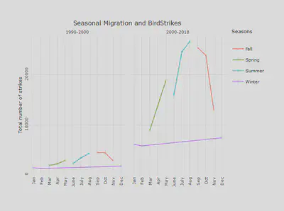
We see here that aside from the increase in birdstrikes in the second period (2000-2018), the usual bird migration seasons Fall and Spring reflect the increase in birds and planes collisions. The Summer season shows a much higher total birdstrikes, this is because some Western Hemisphere bird species also migrate in the summer, or also known as molt migration or postbreeding dispersal. This is true for both Red-tailed Hawks and Gulls that we will see later in our migration analysis.
Flights - Factor 1:
A news article from U.S
Today
reported that there are several factors that contributed to this
increase inplane-bird collisons including “an increase in flights;
changing migratory patterns, etc…”
This is our flight data from 1990 to 2018 obtained from the Department of Transportation for all nonstop commercial passenger traffic traveling between international points and U.S. airports.
#Reading the international dataset
planes <- read.csv("dataset/International_Report_Passengers.csv")

#Filtering for years between 1990 and 2018
planes <- planes %>%
  filter(Year < 2019 & Year >1989)
head(planes)
##     data_dte Year Month usg_apt_id usg_apt usg_wac fg_apt_id fg_apt fg_wac
## 1 09/01/2018 2018     9      99999     ZZZ       1     16310    ZNA    906
## 2 09/01/2018 2018     9      99999     ZZZ       1     16263    YYJ    906
## 3 09/01/2018 2018     9      99999     ZZZ       1     16233    YWH    906
## 4 09/01/2018 2018     9      16744     IL2      41     16271    YYZ    936
## 5 09/01/2018 2018     9      16091     YIP      43     16271    YYZ    936
## 6 09/01/2018 2018     9      15618     VNY      91     16271    YYZ    936
##   airlineid carrier carriergroup       type Scheduled Charter Total
## 1     20272     KAH            1 Passengers         0      20    20
## 2     20272     KAH            1 Passengers         0       1     1
## 3     20272     KAH            1 Passengers         0       3     3
## 4     21437     13Q            0 Passengers         0       4     4
## 5     21437     13Q            0 Passengers         0       4     4
## 6     21352     0WQ            1 Passengers         0      16    16
Let’s aggregate the birdstrike rates for the past 20 years from 1990 to 2018, exluding 2019 due to incomplete year. The number of strikes for each year has increased from approximately 6 strikes/day in 1990 to 46 strikes/day in 2018 if we are to assume 360 days in a year.
#Calculate strike rate for birds
strikerate <- birdstrikes_30yrs %>%
  group_by(INCIDENT_YEAR) %>%
  count() %>%
  mutate(rates = n/360) %>%
  rename(Year = INCIDENT_YEAR)
strikerate$Year <- as.integer(strikerate$Year)
strikerate$label <- "Bird Strikes"

#Calculate flight rate for planes
flightrate <- planes %>%
  count(Year) %>%
  mutate(rates = n/360)
flightrate$label <- "Flights"

#Lets visualize the rates of flight and strikes
bird_flight <- dplyr::bind_rows(strikerate, flightrate)

ani_strikes <- bird_flight %>%
  dplyr::select(Year, rates, label) %>%
  ggplot(aes(x=Year, y=rates, group=label, color=label)) +
  theme_minimal() +
  labs(x = 'Year',
       y = "Rates Per Day") +
  theme(text = element_text(size=16)) +
  ggtitle("Rates of Strikes and Flights from 1990 - 2018") +
  geom_line() +
  geom_point() +
  transition_reveal(Year)

#Make animation and saved as gif
#strike_ani <- gganimate::animate(ani_strikes, 100, 20)
#anim_save(strike_ani)
We can see the increasing trend between the 2 rates. It is explainable by the fact that the birdstrikes data is distributed by the FAA which records each plane-bird collision. We therefore can confirm our first factor: increase in flight -> increase in strikes while holding other factors constant.
Climate - Temperature - Factor 2:
With our confirm assumption that higher birdstrikes happen during bird
migrating seasons, let’s look at how climate temperature can have an
affect on bird activities with.
We are interested in whether hotter months are seen with more
birdstrikes because we suspect that hotter climate means harder
migrations, as stated by PhD student in Biological and Biomedical
Sciences at Harvard Medical
School,
these long migration journey from North to South America in the Fall and
South to North America in the Spring become incredibly dangerous for the
birds. As they might be leaving North America later in the Fall, around
the holiday season for the average American who usually books a flight
to celebrate with family members. These Fall migrating birds therefore
have a higher chance of getting strucks when more planes are on the
air.
Additionally, as the temperature gets hotter, bird species that
rely on the seasonal for food and breeding may arrive earlier in Spring,
as consistent with our earlier observation that more birdstrikes were
seen in May from the 2000 to 2018 period than 1990 - 2000 period. In a
published paper using the same ebird dataset, Hurlbert and
Liang
confirms the early arrival to N.A by 0.8 days for every degree Celcius.
Let’s us take a look at the mean monthly temperatures and strikes for
1990 and 2012 to observe the changes. This is because we would like to
observe a more apparent change and reduce analysis runtime. Since the
data comes in a horizontal format with lats, long that we will be using
for our maps in the later part of this analysis, we will go ahead and
transform the data into a vertical format to compare with our
birdstrikes data. We will do so by transposing the dataframe and find
the mean temperature for each months recorded per year for the U.S.
Notice we are not taking average temperature for the entire America
continent even though our later analysis of migration will be using N.A.
as the scope. This is because birds migrate across the continent for
breeding purposes that tied directly to the opposite nature of
seasonality between North and South America. If you take the average
temperature for N.A. as a whole, we will not be able to see the actual
temperature changes since they be cancelled out by opposite seasonality.
#Function to read and inteprete temperature data
rename_temp <- function(dataset){
  newset <- dataset %>%
    rename(deciLongi = V1,
         deciLatit = V2,
         "1" = V3,
         "2" = V4,
         "3" = V5,
         "4" = V6,
         "5" = V7,
         "6" = V8,
         "7" = V9,
         "8" = V10,
         "9" = V11,
         "10" = V12,
         "11" = V13,
         "12" = V14)
  return(newset)
}

temp1990 <- rename_temp(read.table("dataset/air_temp1990.txt")[1:14])
temp2012 <- rename_temp(read.table("dataset/air_temp2012.txt")[1:14])
head(temp1990)
##   deciLongi deciLatit     1     2     3     4    5   6   7   8    9    10
## 1   -179.75     71.25 -24.8 -30.1 -24.7 -12.7 -2.5 0.6 2.2 4.3 -0.7  -6.0
## 2   -179.75     68.75 -30.1 -32.5 -22.5 -11.5 -3.8 0.8 3.0 3.7 -0.9  -8.7
## 3   -179.75     68.25 -30.5 -34.4 -24.0 -12.9 -4.4 1.2 3.5 4.1 -1.4  -9.5
## 4   -179.75     67.75 -28.9 -35.1 -24.2 -12.7 -3.1 4.0 6.7 6.8 -0.1  -8.8
## 5   -179.75     67.25 -30.9 -39.2 -27.6 -15.7 -5.0 3.8 6.9 6.4 -1.8 -11.7
## 6   -179.75     66.75 -26.8 -35.0 -23.6 -12.7 -2.6 5.6 9.0 8.8  0.6  -8.7
##      11    12
## 1 -15.3 -25.6
## 2 -16.8 -27.7
## 3 -18.1 -28.1
## 4 -18.1 -26.7
## 5 -21.5 -29.1
## 6 -18.2 -24.4
#function that reformat the temperatures filtered by the American continent
my_transpose <- function(data){
  trans <- data %>%
   filter(deciLongi >= -125.0011,
           deciLongi <= -66.9326,
           deciLatit >= 24.9493,
           deciLatit <= 50.0704) %>%
  subset(select = -c(deciLongi, deciLatit)) %>%
  lapply(mean) %>%
  as.data.frame(long=TRUE) %>%
  gather() %>%
  rename(Month =  key, Celcius = value)
  return(trans)
}

#transposing into vertical format
summary_temp90 <- my_transpose(temp1990)
summary_temp12 <- my_transpose(temp2012)

#Monthly strikes
temp_strikes_12 <- birdstrikes_10yrs_2 %>%
  filter(INCIDENT_YEAR==2012) %>%
  cbind(ave_temp = round(((summary_temp12$Celcius*9/5)+32), 3))

temp_strikes_19 <- birdstrikes_10yrs_1 %>%
  filter(INCIDENT_YEAR==1990) %>%
  cbind(ave_temp = round(((summary_temp90$Celcius*9/5)+32), 3))
head(temp_strikes_19)
## # A tibble: 6 x 6
## # Groups:   INCIDENT_MONTH [6]
##   INCIDENT_MONTH INCIDENT_YEAR     n label     Seasons ave_temp
##            <dbl>         <dbl> <int> <chr>     <chr>      <dbl>
## 1              1          1990    36 1990-2000 Winter      34.4
## 2              2          1990    31 1990-2000 Winter      33.6
## 3              3          1990    33 1990-2000 Spring      42.4
## 4              4          1990    63 1990-2000 Spring      51.1
## 5              5          1990   231 1990-2000 Spring      57.7
## 6              6          1990   162 1990-2000 Summer      68.9
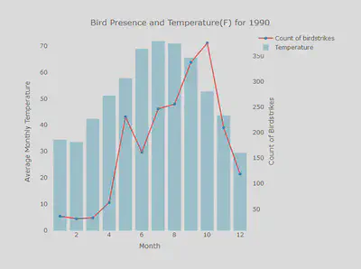
Now that we have our temperatures formatted and converted into Fahenheit. Let see what relationship exists between strikes and temperature in the U.S. for the years of 1990 and 2000.
#create axis layouts, explicitly
R_Axis <- list(side = "right", overlaying = "y", title ="Count of Birdstrikes", showgrid = FALSE, zeroline = FALSE)
L_Axis <- list(side = "left", title ="Average Monthly Temperature", showgrid = FALSE, zeroline = FALSE)

one_plot <- function(data) {
  data %>% plot_ly(x = data$INCIDENT_MONTH) %>%
  add_trace(y = ~n,
            name = 'Count of birdstrikes',
            type = 'scatter',
            mode = "markers",
            yaxis = 'y2',
            line = list(color = "red"),
            hoverinfo = "text",
            text = ~paste(n, "Strikes")) %>%
  add_trace(y = ~ave_temp, type = 'bar', name = "Temperature",
            yaxis = 'y',
            marker = list(color = 'lightblue'),
            hoverinfo = "text",
            text = ~paste(ave_temp, 'F')) %>%
    layout(title = "Bird Presence and Temperature(F) for 1990 and 2012",
          xaxis = list(title = "Month"),
          yaxis2 = R_Axis,
          yaxis = L_Axis)
}

p1 <- one_plot(temp_strikes_19)
p1 %>%
  layout(title = "Bird Presence and Temperature(F) for 1990")
## A line object has been specified, but lines is not in the mode
## Adding lines to the mode...
#There is a bug in plotly subplot, for this reason we will view them separately.
p2 <- one_plot(temp_strikes_12)
p2 %>%
  layout(title = "Bird Presence and Temperature(F) for 2012")
## A line object has been specified, but lines is not in the mode
## Adding lines to the mode...
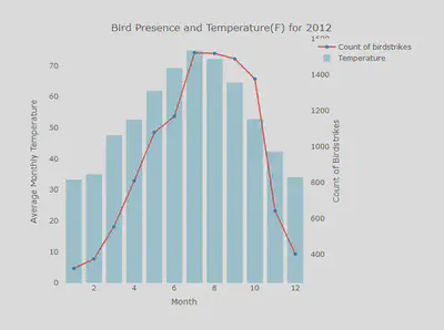
It seems to show from our two plots that increasing temperature is not
associated with increasing birdstrikes. The higher birdstrikes in 2012
increased from Aug to Nov. This can affirm our suspicion that birds more
birds are leaving later in the Fall and higher number of planes in the
air during the holiday seasons can mean higher probability of their
collisions. We cannot however, confirm the other hypothesis that higher
temperature lead to changes in bird migration pattern as did our
referred paper.
Again, these are not direct correlation and we
cannot uncertain that flight or temperature alone can cause birdstrikes
to increase. This is why we are going to look at birth migration as our
next factor.
Bird Migration - Factor 3:
Here is the NOAA Wester Hemisphere bird migration patterns:
We would like to replicate this pattern for our selected species.
To dig deeper into these reasons, why have acquired the bird migration
data from the ebird database. We will focus on the migration pattern of
the top 10 species of birds that are most frequently striked up to
date.
We chose to analyze the following years to observe changes in migration
pattern: 1990 and 2012 due to the availability of the original ebird
data for our selected species.
To select our species, we chose the most struck bird species except for
the species listed as unknown. Those species are: Morning dov, Gulls,
Killdeer, Barn swallow, Horned lark, European staling, Sparrows, Rock
pigeon, Red-tailed hawk, Eastern meadowlark.
# Showing the top birds being struck
total_species <- birdstrikes %>%
  group_by(SPECIES) %>%
  summarize(total_count_species = n()) %>%
  arrange(desc(total_count_species, decl))
head(total_species,20)
## # A tibble: 20 x 2
##    SPECIES               total_count_species
##    <chr>                               <int>
##  1 Unknown bird - small                40971
##  2 Unknown bird - medium               40537
##  3 Unknown bird                        13644
##  4 Mourning dove                       10706
##  5 Gulls                                7178
##  6 Killdeer                             6635
##  7 Barn swallow                         6332
##  8 American kestrel                     6244
##  9 Horned lark                          5739
## 10 European starling                    4897
## 11 Sparrows                             3642
## 12 Rock pigeon                          3481
## 13 Unknown bird - large                 3304
## 14 Red-tailed hawk                      3110
## 15 Eastern meadowlark                   2930
## 16 Cliff swallow                        2191
## 17 Ring-billed gull                     1851
## 18 Canada goose                         1822
## 19 Western meadowlark                   1733
## 20 American robin                       1595
Those birds are seen in North America based on the FAA birdstrike data of strikes in U.S airports. We suspect that they migrate North to South America as they are Western Hemisphere birds. Below are some information about the birds we work with.
| Species | Migration Patterns | Status |
|---|---|---|
| Mourning Dove | Columbidae | Resident to long-distance migrant. Northern birds fly south thousands of miles (as far as southern Mexico); individuals that breed in central and southern U.S. move a few hundred miles or not at all. |
| Gulls | Laridae | Regular seasonal migration to and from Pacific Coast. Vast majority leave breeding grounds in late summer, flying to Pacific Coast to spend nonbreeding months. In contrast to other large white-headed gulls, few individuals remain in breeding range during nonbreeding season. |
| Kill Deer | Charadriidae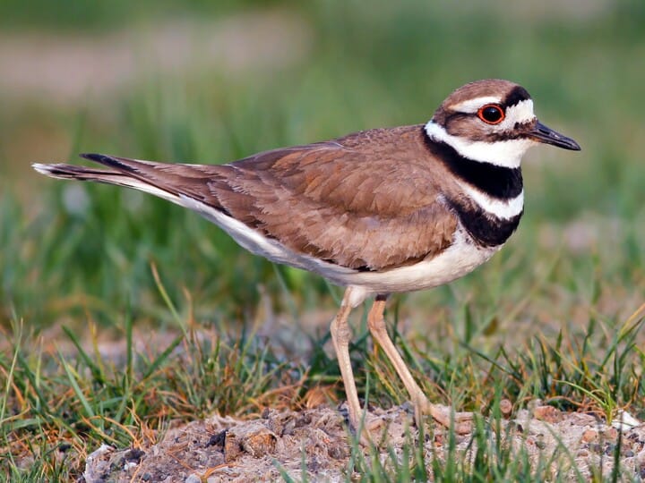 | Resident or medium-distance migrant. Some northern birds spend the winter in Mexico. In the southern United States and Pacific coast, Killdeer are year-round residents. |
| Barn Swallow | Hirundo rustica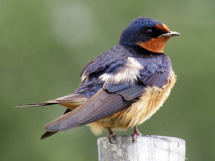 | Long-distance migrant. Barn Swallows fly from North American breeding grounds to wintering areas in Central and South America. Southbound fall migration may begin by late June in Florida or early July in Massachusetts. They return as early as late January in southern California to mid-May at Alaskan breeding sites. |
| American Kestrel | Falco sparverius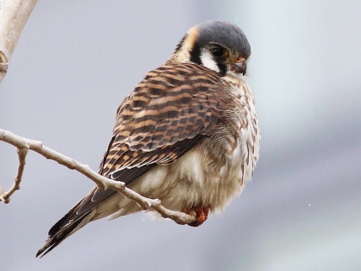 | Resident to long-distance migrant. In North America, the tendency for kestrels to migrate decreases from north to south, with southernmost populations resident year-round. While some American Kestrels migrate to Central America, the great majority spend the winter in the southern United States. Kestrels can often be seen along mountain ridges and at hawk watches during fall migration. |
| Horned Lark | Eremophila alpestris | Resident to short-distance migrant. Populations breeding in northern North America move south into Lower 48 for winter; other populations are resident year-round. Migrates by day in flocks, foraging on the move. Alpine-breeding populations move to surrounding lowlands in winter. |
| European Starling | Sturnus vulgaris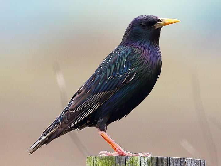 | Resident to short-distance migrant. Adult birds north of 40 degrees (the latitude of New York City) and many juveniles move south in winter, traveling down river valleys or along the coastal plains. Some birds spend the winter in northern Mexico and the Lesser Antilles, but most remain in continental North America. |
| Sparrows | Passerellidae | Resident to medium-distance migrant. Birds from far Alaska and northern Canada migrate the farthest, flying to the southern United States and northern Mexico to winter. Birds from the northern U.S. may migrate, but typically don’t go as far south as the birds that started from farther north, a pattern called “leapfrog migration.” |
| Red-tailed hawk | Buteo jamaicensis | Resident or short-distance migrant. Most birds from Alaska, Canada, and the northern Great Plains fly south for a few months in winter, remaining in North America. Birds across the rest of the continent typically stay put, sharing the countryside with northern arrivals. |
| Eastern meadowlark | Sturnella magna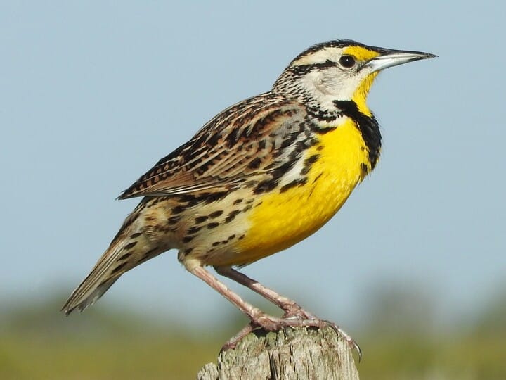 | Resident to short-distance migrant, although some birds from northern populations migrate more than 600 miles to the southern U.S. These migrating meadowlarks typically depart by the end of November for wintering areas and return to the north after the snow melts in spring. |
In order to recreate these birds migration patterns along with monthly temperatures for 1990 and 2012 as we did earlier for our temperature and strike analysis, we will need to reformat our temperature data again to filter by the bounding box of the North America because these bird species migrate across the continent. After that we will take the mean temperatures for each month and year.
# Creatign one large dataset from the two temperature periods
#this is our North America bounding box based on lat, lon google coordinates (y, x)
#coord_sf(xlim = c(-130.85, -29.78), ylim = c(51.97,-57.86), expand =F)

round_temp <- function(dataset, year) {
  new_temp <- dataset %>%
    filter(deciLongi >= -130.85,
           deciLongi <= -29.78,
           deciLatit >= -57.86,
           deciLatit <= 51.97) %>%
    gather("month", "temperature", 3:14) %>%
    mutate(year = year) %>%
    mutate(deciLongi = round(deciLongi, 2),
           deciLatit = round(deciLatit, 2)
           ) %>%
    group_by(deciLongi, deciLatit, month, year) %>%
    summarise(tempmean = mean(temperature)
              ) %>%
    ungroup()
  return(new_temp)
}

temp_round19 <- round_temp(temp1990, 1990)
temp_round12 <- round_temp(temp2012, 2012)
temperatures <- rbind(temp_round19, temp_round12)
head(temperatures)
## # A tibble: 6 x 5
##   deciLongi deciLatit month  year tempmean
##       <dbl>     <dbl> <chr> <dbl>    <dbl>
## 1     -128.      50.8 1      1990      4.8
## 2     -128.      50.8 10     1990      8.7
## 3     -128.      50.8 11     1990      6
## 4     -128.      50.8 12     1990      2.6
## 5     -128.      50.8 2      1990      3.3
## 6     -128.      50.8 3      1990      6.2
temp <- stack()
for (i in 1:12) {
    x1 <- rasterFromXYZ(temperatures %>%
                          filter(year == 1990 & month == i) %>%
                          select(deciLongi, deciLatit, tempmean)
    )
    names(x1) <- paste0("Temperature ",i,", 1990")
      temp <- stack(temp, x1)
}
for (i in 1:12) {
    x1 <- rasterFromXYZ(temperatures %>%
                          filter(year == 2012 & month == i) %>%
                          select(deciLongi, deciLatit, tempmean)
    )
    names(x1) <- paste0("Temperature ",i,", 2012")
      temp <- stack(temp, x1)
}
Here is the subsetted ebird data filtered from a cloud server. On this server, we summed up the count of the column individualCount which lists how many of the specific species is seen per location. We set NA values for the individualCount column to be 1 because we assume that every observation contains at least 1 bird.
# Reading into the xported subsetted ebird dataset generated from an online server
subsetted <- readRDS("dataset/ebirdsubset.rds")

migration <- subsetted %>%
  filter(decimalLongitude >= -130.85,
         decimalLongitude <= --29.78,
         decimalLatitude >= -57.86,
         decimalLatitude <= 51.97, #Filtering for points within the United States bounding box
         family == "Columbidae" |
           family == "Laridae" |
           family == "Charadriidae"|
           scientificName== "Hirundo rustica"|
           scientificName == "Falco sparverius" |
           scientificName == "Eremophila alpestris" |
           scientificName == "Sturnus vulgaris" |
           family == "Passeridae" |
           scientificName == "Buteo jamaicensis" |
           scientificName == "Sturnella magna"
         )%>% # fine grain filtering for required species
  mutate(species = case_when(
     family == "Columbidae" ~ "Mourning Dove",
     family == "Laridae" ~ "Gulls",
     family == "Charadriidae" ~ "Kill Deer",
     scientificName== "Hirundo rustica" ~ "Barn Swallow",
     scientificName == "Falco sparverius" ~ "American Kestrel",
     scientificName == "Eremophila alpestris" ~ "Horned Lark",
     scientificName == "Sturnus vulgaris" ~ "European Starling",
     family == "Passeridae" ~ "Sparrows",
     scientificName == "Buteo jamaicensis"~"Red-tailed hawk",
     scientificName == "Sturnella magna" ~ "Eastern meadowlark",
    ) # renaming species with common names to match with strike dataset
)

head(migration)
## # A tibble: 6 x 8
## # Groups:   decimalLatitude, decimalLongitude, scientificName, family,
## #   month [6]
##   decimalLatitude decimalLongitude scientificName family month  year
##             <dbl>            <dbl> <chr>          <chr>  <chr> <dbl>
## 1           -53.2            -70.7 Larus dominic~ Larid~ 02     1990
## 2           -53.2            -70.7 Sterna hirund~ Larid~ 02     1990
## 3           -53.2            -70.9 Chroicocephal~ Larid~ 02     1990
## 4           -53.2            -70.9 Columba livia  Colum~ 02     1990
## 5           -53.2            -70.9 Falco sparver~ Falco~ 02     1990
## 6           -53.2            -70.9 Larus dominic~ Larid~ 02     1990
## # ... with 2 more variables: TotalCounts <dbl>, species <chr>
Here will obtain the migration locations for each species as points by weighing the total observations at a coordinate for every month every year. Our group acknowledges that there are more sophisticated methods, and there may be errors associated with averaging over independent longitude and latitudes, but considering that we are only interested in the highest density of points and that data was aggregated over a span of one month, the summary method is sufficient for the species we are interested in.
migsums <- migration %>%
  ungroup() %>%
  group_by(species, month, year) %>%
  summarize(mlongi = sum(decimalLongitude*TotalCounts)/sum(TotalCounts),
         mlatit = sum(decimalLatitude*TotalCounts)/sum(TotalCounts))

tempPOSI <- temperatures %>%
  mutate(date = as.Date(paste(year,month,"01"), "%Y%m%d", tz="UTC")) %>%
  mutate(date = as.POSIXct(date, tz = "UTC"))

migraPOSI <- migsums %>%
  mutate(date = as.Date(paste(year,month,"01"),  "%Y%m%d", tz="UTC")) %>%
  mutate(date = as.POSIXct(date, tz = "UTC"))

projection <- "+proj=longlat +datum=WGS84 +no_defs"

#Creating frames for 1990
migrmove90 <- df2move(filter(migraPOSI, year == 1990),
        proj=projection,
        x= "mlongi",
        y="mlatit",
        time= "date",
        track_id = "species")

migrmove90 <- align_move(migrmove90, res = 10, digit = 0, unit = "days")

frames90 <- frames_spatial(migrmove90,
                           path_colours = c("#e6194B", "#3cb44b", "#ffe119", "#4363d8", "#f58231", "#911eb4", "#42d4f4", "#f032e6", "#bfef45", "#fabebe"),
                           map_service = "mapbox",
                           map_type = "satellite",
                           map_token = "pk.eyJ1IjoiYWxpY2VodWExMSIsImEiOiJjam1iMHV5aXAwMGRtM3JzM2dzamJjamkzIn0.gCsvu2g9o3J5DKJfNarokQ",
                           alpha = 0.5) %>%
  add_labels(x = "Longitude", y = "Latitude") %>% # add some customizations, such as axis labels
  add_northarrow() %>%
  add_scalebar() %>%
  add_timestamps(type = "label") %>%
  add_progress()
## Checking temporal alignment...
## Processing movement data...
## Approximated animation duration: ˜ 1.2s at 25 fps for 30 frames
## Retrieving and compositing basemap imagery...
## Assigning raster maps to frames...
## Creating frames...
#saving animation for 1990
#animate_frames(frames90, out_file = "image/migration19.gif", fps=100, overwrite = T)

#Creating frames for 2012
migrmove12 <- df2move(filter(migraPOSI, year==2012),
        proj=projection,
        x= "mlongi",
        y="mlatit",
        time= "date",
        track_id = "species")

migrmove12 <- align_move(migrmove12, res = 10, digit = 0, unit = "days")

frames12 <- frames_spatial(migrmove12,
                           path_colours = c("#e6194B", "#3cb44b", "#ffe119", "#4363d8", "#f58231", "#911eb4", "#42d4f4", "#f032e6", "#bfef45", "#fabebe"),
                           map_service = "mapbox",
                           map_type = "satellite",
                           map_token = "pk.eyJ1IjoiYWxpY2VodWExMSIsImEiOiJjam1iMHV5aXAwMGRtM3JzM2dzamJjamkzIn0.gCsvu2g9o3J5DKJfNarokQ",
                           alpha = 0.5)%>%
  add_labels(x = "Longitude", y = "Latitude") %>% # add some customizations, such as axis labels
  add_northarrow() %>%
  add_scalebar() %>%
  add_timestamps(type = "label") %>%
  add_progress()
## Checking temporal alignment...
## Processing movement data...
## Approximated animation duration: ˜ 1.08s at 25 fps for 27 frames
## Retrieving and compositing basemap imagery...
## Assigning raster maps to frames...
## Creating frames...
#saving animation for 2012
#animate_frames(frames12, out_file = "image/migration12.gif", fps=100, overwrite = T)

Looking at the migration patterns for 1900 and 2012, we can see that
migration patterns became more local to only North America while the
patterns for 1990 spand across are what we expected. We went back to
double check that our bounding box is correctly placed over the entire
America continent and that both years of analysis are contained in one
table. This is a surprise to us and we suspect that bird species could
have adapted to urban living or shorter migration paths in the age of
warming climate.
Here we run a Mutiple Poisson Regression to see the
overall effects that planes and temperatures have on bird strikes.
reg <- birdstrikes %>%
  select(INCIDENT_MONTH, INCIDENT_YEAR) %>%
  filter(INCIDENT_YEAR == 2012|
           INCIDENT_YEAR == 1990) %>%
  mutate(Strike = 1) %>%
  group_by(INCIDENT_MONTH, INCIDENT_YEAR) %>%
  summarise(Strike = sum(Strike)) %>%
  rename(month = INCIDENT_MONTH,
         year = INCIDENT_YEAR) %>%
  left_join(
    (temperatures %>%
      select(month, year, tempmean) %>%
      group_by(month, year) %>%
      summarize(mtemp = mean(tempmean)) %>%
      ungroup() %>%
      mutate_at(vars(month), as.numeric)
    ), by=c("month", "year")
  ) %>%
  left_join(
    (planes %>%
      select(Year, Month, Total) %>%
       filter(Year == 2012 |
                Year == 1990) %>%
       rename(year = Year,
              month = Month) %>%
       group_by(year, month) %>%
       summarize(planes = sum(Total))
    )
  ) %>%
  left_join(
    (migration %>%
      ungroup() %>%
      select(month, year, TotalCounts) %>%
      group_by(month, year) %>%
      count() %>%
      ungroup() %>%
      mutate_at(vars(month), as.numeric) %>%
      rename(birds = n)
    )
  )
## Joining, by = c("month", "year")Joining, by = c("month", "year")
reg <- reg %>%
  dummy_cols("month",
             remove_first_dummy = T) %>%
  dummy_cols("year",
             remove_first_dummy = T)
rreg<- glm(formula = Strike ~ mtemp + planes + month_2+month_3+month_4+month_5+month_6+month_7+month_8+month_9+month_10+month_11+month_12+year_2012, family = "poisson", data = reg)
summary(rreg)
##
## Call:
## glm(formula = Strike ~ mtemp + planes + month_2 + month_3 + month_4 +
##     month_5 + month_6 + month_7 + month_8 + month_9 + month_10 +
##     month_11 + month_12 + year_2012, family = "poisson", data = reg)
##
## Deviance Residuals:
##     Min       1Q   Median       3Q      Max
## -7.1390  -1.9118  -0.1045   2.4823   4.5818
##
## Coefficients:
##              Estimate Std. Error z value Pr(>|z|)
## (Intercept) 1.894e+00  7.179e-01   2.638 0.008335 **
## mtemp       8.111e-02  6.375e-02   1.272 0.203248
## planes      1.878e-07  4.140e-08   4.536 5.72e-06 ***
## month_2     3.651e-01  9.489e-02   3.848 0.000119 ***
## month_3     4.569e-02  1.771e-01   0.258 0.796407
## month_4     4.449e-01  2.325e-01   1.913 0.055731 .
## month_5     6.851e-01  3.240e-01   2.114 0.034488 *
## month_6     3.575e-01  3.819e-01   0.936 0.349199
## month_7     3.071e-01  4.225e-01   0.727 0.467312
## month_8     3.333e-01  4.465e-01   0.746 0.455407
## month_9     9.656e-01  4.232e-01   2.282 0.022512 *
## month_10    1.191e+00  2.857e-01   4.168 3.07e-05 ***
## month_11    7.675e-01  1.619e-01   4.739 2.14e-06 ***
## month_12    2.311e-01  7.604e-02   3.039 0.002377 **
## year_2012   2.108e-01  2.938e-01   0.717 0.473171
## ---
## Signif. codes:  0 '***' 0.001 '**' 0.01 '*' 0.05 '.' 0.1 ' ' 1
##
## (Dispersion parameter for poisson family taken to be 1)
##
##     Null deviance: 10707.7  on 23  degrees of freedom
## Residual deviance:   249.7  on  9  degrees of freedom
## AIC: 462.38
##
## Number of Fisher Scoring iterations: 4
rreg$coefficients
##  (Intercept)        mtemp       planes      month_2      month_3
## 1.894072e+00 8.111163e-02 1.877998e-07 3.651206e-01 4.568683e-02
##      month_4      month_5      month_6      month_7      month_8
## 4.448965e-01 6.851430e-01 3.575383e-01 3.071298e-01 3.332660e-01
##      month_9     month_10     month_11     month_12    year_2012
## 9.656213e-01 1.190870e+00 7.675005e-01 2.310559e-01 2.107561e-01
The coefficient for planes is positive overall, but we notice that for every additional plane to enter the skies, there is a 0.00000015 chance for a bird to be struck. This supports our theory that there are other variables at play. We notice that the most significant coefficient is the dummy controlling for year_2012. This finding has several implications, though the most jarring is that birds are becoming more at risk as we enter the future. It’s also interesting to note that the individual month dummies have vastly different coefficients, some negative and positive. Interstingly, april, may, september, october, november, december report the highest coefficient values, which support our hypothesis that birds are most at risk during the migratory months.
It’s important to note that our method of running this analysis is compling the month and years from each account and averaging them. While this simple regression is helpful to understand some elementary trends from our data, it should not be relied upon. Many coefficients have insiginificant p-values associated with them, so it is important to note that an enriched dataset and more observations will be more helpful in understanding the true effects of these variables on strikes.
Conclusion
Flights takeoffs and bird migration are two important aspects of bird
strikes, and our analysis showed that these are two aspects that we
should keep in mind as we move into a future of increased air travel and
shifting migration patterns. In this study, we aim to analysis the
factors that contribute to bird strikes to answer a few fundamental
questions such as what is the bird strike trend, when do they take place
most, what is the relationship between the strikes and flights, climate
change, bird migration patterns.
We made a general assumption that high bird strikes indicate high bird
species presence. In general, the usual Fall and Spring migration
patterns are correlated to higher strike counts. We then analyzed data
about bird strikes for the last 28 years for general observation.
Generally, more bird and plane collisions happen throughout the year
with an emphasis on higher strikes from April to Nov. By splitting the
data into 2 different periods, 1990 -2000 and 200 - 2018, we observe
higher bird strikes in the last 18 years where May in particular has
more strikes than the previous 10-year period. A more detailed analysis
showed that strikes usually take place during bird migration seasons,
from early Spring to late Fall.We also suspect that climate change is
changing the bird migration patterns and hence their activities which
leads to changing number of bird strikes.
Analysis of our first factor indicated a correlation between the rate of
strikes and the rate of plane take-offs. Not surprisingly, more planes
in the air means more birds are at risk of getting struck, and the data
shows that they do get struck.
Analysis of our second factor using
two years 1990 and 2012 indicates that temperature do not directly
correlated to higher bird strikes although the referred paper confirmed
the earlier arrival of birds in Spring. The increase in strikes from Aug
to Nov could be however, suspected to be caused by later Fall migration
which is a seasonal shift caused by warmer climate.
Analysis of our third and most important factor: bird migration pattern
in 1990 and 2012 where the 10 selected birds based on their highest
strike record. Our visualization shows that they are becoming long-term
residents of a location or also known as resident birds. The prime
example is the well-known pigeon. This species, also in the family of
doves, is among the variety that we notice are becoming static. Yet this
isn’t a new trend.
Researchers are
beginning to notice this pattern in a variety of species.
In a 2010
study of migratory evolution, Francisco Pulido and Peter Berthold
suggests:
Our findings suggest that current alterations of the environment are favoring birds wintering closer to the breeding grounds and that populations of migratory birds have strongly responded to these changes in selection. The reduction of migratory activity is probably an important evolutionary process in the adaptation of migratory birds to climate change, because it reduces migration costs and facilitates the rapid adjustment to the shifts in the timing of food availability during reproduction.
Overall, we find that bird strikes are positively correlated with flights but not temperature. We also find a local migration pattern for the birds that most striked at U.S airports. While this module has not specifically explored the impacts of climate change on bird strikes, it has pointed clearly to the increasing number of birds being struck as a result of urbanization.
Further research:
I’ve conducted a Suitability Analysis for Professor Jasenka Rakas from the Civil and Environment Department at UC Berkeley to look at the potential locations for future vertiports. Using cartographic and gis tools, here is what we found: